Keywords: Parametic Polynomial Curves, Bezier Curves, Spline Curves, Subdivision, C++
This is the Chapter13 ReadingNotes from book 3D Math Primer for Graphics and Game Development 2nd Edition.
Parametic Polynomial Curves
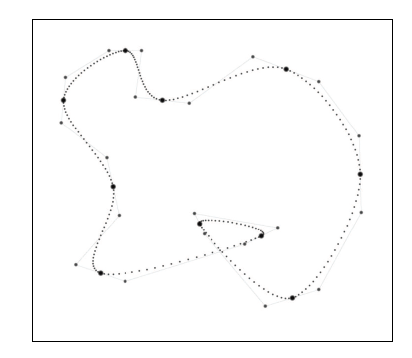
Parametric Curves
The word parametric in the phrase “parametric polynomial curve” means that the curve can be described by a function of an independent paramete, which is often assigned the symbol $t$. This curve function is of the form $p(t)$, taking a scalar input (the parameter $t$) and returning the point on the curve corresponding to that parameter value as a vector output. The function $p(t)$ traces out the shape of the curve as $t$ varies.
implicit: $x^2 + y^2 = 1$, explicit: $y = \sqrt{1-x^2}$
parametric:
$$
\vec{p(t)} = (x(t), y(t))\\
\begin{cases}
x(t) = \cos(2\pi t)\\
y(t) = sin(2\pi t)
\end{cases}
$$
Polynomial Curves(多项式曲线)
The number $n$ is called the degree of the polynomial.
$$
\vec{p(t)} = \vec{c_0} + \vec{c_1}t + \vec{c_2}t^2 + \cdots + \vec{c_{n-1}}t^{n-1} + \vec{c_n}t^n
$$
Cubic Curve in Monomial Form
$$
\vec{p(t)} = \vec{c_0} + \vec{c_1}t + \vec{c_2}t^2 + \vec{c_3}t^3
\tag{13.2}
$$
Matrix Notation
2D cubic curve in expanded monomial form:
$$
\begin{cases}
x(t) = c_{1,0} + c_{1,1}t + c_{1,2}t^2 + c_{1,3}t^3\\
y(t) = c_{2,0} + c_{2,1}t + c_{2,2}t^2 + c_{2,3}t^3
\end{cases}
$$
thus,
$$
\begin{aligned}
\vec{p(t)} = C\vec{t} &=
\begin{bmatrix}
c_{1,0} & c_{1,1} & c_{1,2} & c_{1,3}\\
c_{2,0} & c_{2,1} & c_{2,2} & c_{2,3}
\end{bmatrix}
\begin{bmatrix}
1 \\ t \\ t^2 \\ t^3
\end{bmatrix}\\
&=
\begin{bmatrix}
\vec{c_0} &\vec{c_1} & \vec{c_2} & \vec{c_3}
\end{bmatrix}
\begin{bmatrix}
1 \\ t \\ t^2 \\ t^3
\end{bmatrix}
\end{aligned}
$$
Two Trivial Types of Curves
Consider a ray from the point $p_0$ to the point $p_1$. If we let $\vec{d}$ be the delta vector $\vec{p_1} − \vec{p_0}$, then the ray is expressed parametrically as
$$
\vec{p(t)} = \vec{p_0} + \vec{d}t
\tag{13.3}
$$
let $\vec{c_0} = \vec{p_0}$, $\vec{c1} = \vec{d}$,this linear curve is a polynomial curve of degree 1.
Endpoints in Monomial Form
Suppose, $0 \leq t \leq 1$, start and end points are $\vec{p(0)}$ and $\vec{p(1)}$.
$c_0$ specifies the start point; The endpoint is the sum of the coefficients.
$$
\begin{aligned}
&\vec{p_0} = \vec{c_0}\\
&\vec{p_1} = \vec{c_0} + \vec{c_1} + \vec{c_2} + \vec{c_3}
\end{aligned}
$$
Velocities and Tangents
the velocity function $v(t)$ is the first derivative of the position function $p(t)$ because velocity measures the rate of change in position over time. Likewise, the acceleration function $a(t)$ is the derivative of the velocity function $v(t)$ because acceleration measures the rate of change of velocity over time.
Velocity and Acceleration of Cubic Monomial Curve
$$
\vec{p(t)} = \vec{c_0} + \vec{c_1}t + \vec{c_2}t^2 + \vec{c_3}t^3
\tag{13.4}
$$
$$
\vec{v(t)} = \dot{\vec{p(t)}} = \vec{c_1} + 2\vec{c_2}t + 3\vec{c_3}t^2
\tag{13.5}
$$
$$
\vec{a(t)} = \ddot{\vec{p(t)}} = 2\vec{c_2} + 6\vec{c_3}t
\tag{13.6}
$$
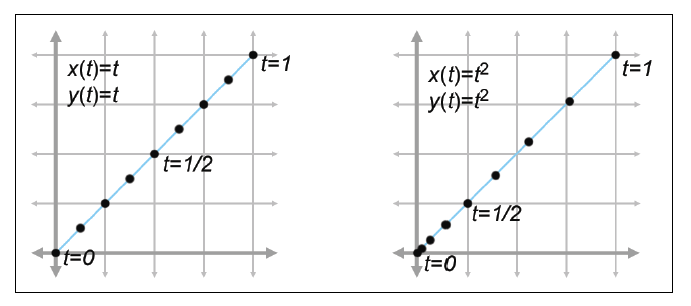
Two curves that define the same “shape,” but not the same “path”:
$$
p(t) = p_0 + dt
$$
$$
Let \space s(t) = t^2 \mapsto p(s(t)) = p_0 + dt^2
$$
The tangent at a point is the direction the curve is moving at that point, the line that just touches the curve. The tangent is basically the normalized velocity of the curve.
$$
\vec{t(t)} = \widehat{\vec{v(t)}} = \frac{\vec{v(t)}}{||\vec{v(t)}||}
$$
The second derivative is related to curvature, which is sometimes denoted $\kappa$,
$$
\vec{\kappa(t)} = \frac{||\vec{v(t)} \times \vec{a(t)}||}{||\vec{v(t)}||^3}
$$
Polynomial Interpolation
linear interpolation: Given two “endpoint” values, create a function that transitions at a constant rate (spatially, in a straight line) from one to the other (is simply first-degree polynomial interpolation).
Polynomial interpolation: Given a series of control points, our goal is to construct a polynomial that interpolates them.
A polynomial of degree $n$ can be made to interpolate $n + 1$ control points.
We use the word “knot” to refer to control points that are interpolated, invoking the metaphor of a rope with knots in it.
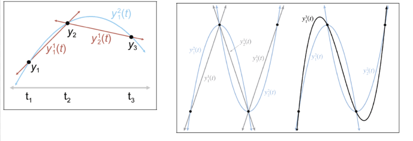
Aitken’s Algorithm(Geometry View)
recursive algorithms, divide and conquer.
To solve a difficult problem, we first divide it into two (or more) easier problems, solve the easier problems independently, and then combine the results to get the solution to the harder problem.
We split this curve into two “easier” curves: (1) one that interpolates only the first $n − 1$ points, disregarding the last point; and (2) another that interpolates the last $n − 1$ points without worrying about the first point. Then, we blend these two curves together.
We let $y_i^1(t)$ denote the linear curve between $y_i$ and $y_{i+1}$, the notation $y_i^2(t)$ denote the quadratic curve between $y_i$ and $y_{i+2}$, and so on
Linear interpolation between two control points:
$$
y_1^1(t) = \frac{(t_2 - t)y_1 + (t - t_1)y_2}{t_2 - t_1}
$$
$$
y_2^1(t) = \frac{(t_3 - t)y_2 + (t - t_2)y_3}{t_3 - t_2}
$$
Linear interpolation of lines yields a quadratic curve
$$
y_1^2(t) = \frac{(t_3 - t)[y_1^1(t)] + (t - t_1)[y_2^1(t)]}{t_3 - t_1}
$$
Lagrange Basis Polynomials(Math View)
Each control point gives us one equation, and each coefficient gives us one unknown. This system of equations can be put into an $n \times n$ matrix, which can be solved by standard techniques such as Gaussian elimination or 👉$LU$ decomposition.
we could create a polynomial for each knot $t_i$ such that the polynomial evaluates to unity at that knot, but for all the other knots it evaluates to zero.
$$
\zeta_1(t_1) = 1, \zeta_2(t_1) = 1, \zeta_3(t_1) = 1, \zeta_4(t_1) = 1\\
\cdots \\
\zeta_1(t_4) = 0, \zeta_2(t_4) = 0, \zeta_3(t_4) = 0, \zeta_4(t_4) = 1\\
$$
Interpolating polynomial in Lagrange basis form
$$
p(t) = \sum_{i=1}^n y_i\zeta_i(t) =
y_1\zeta_1(t) + y_2\zeta_2(t) + \cdots + y_3\zeta_3(t)
\tag{13.7}
$$
Lagrange Basis Polynomial
$$
\zeta_i(t) = \prod_{1 \leq j \leq n, j \neq i} \frac{t - t_i}{t_i - t_j}
$$
Thus, we could calculate:
$$
\zeta_1(t) = -(\frac{9}{2})t^3 + 9t^2 - (\frac{11}{2})t + 1
$$
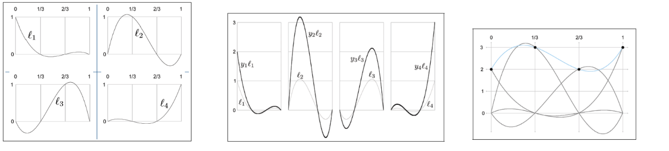
we scale each basis polynomial by the corresponding coordinate value, adding the scaled basis vectors together yields the interpolating polynomial $P$.
$$
\begin{aligned}
P(t) &= y_1\zeta_1(t) + y_2\zeta_2(t) + \cdots + y_3\zeta_3(t)\\
&= 18t^3 − 27t^2 + 10^t + 2.
\end{aligned}
$$
We can think of basis polynomials as functions yielding barycentric coordinates (blending weights).
view1: the control points are the building blocks and the basis polynomials provide the scale factors, although we prefer to be more specific and call these scale factors barycentric coordinates.
view2: any arbitrary vector can be described as a linear combination of the basis vectors. In our case, the space being spanned by the basis is not a geometric 3D space, but the vector space of all possible polynomials of a certain degree, and the scale values for each curve are the known values of the polynomial at the knots.
👉More about Curve Fitting in PatternRecognition>>
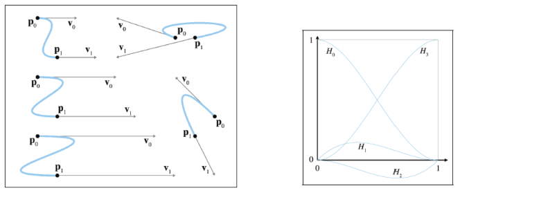
Hermite Curves
Polynomial interpolation doesn’t work as well as we would like, because of the tendency to oscillate and overshoot, so let’s try a different approach.
Instead of specifying the interior positions to interpolate, let’s control the shape of the curve through the tangents at the endpoints.
System of equations for Hermite conditions (cubic curve)
$$
\begin{aligned}
&p(0) = p_0 \Longrightarrow c_0 = p_0\\
&v(0) = v_0 \Longrightarrow c_1 = v_0\\
&v(1) = v_1 \Longrightarrow c_1 + 2c_2 + 3c_3 = v_1\\
&p(1) = p_1 \Longrightarrow c_0 + c_1 + c_2 + c_3 = p_1
\end{aligned}
$$
Converting Hermite form to monomial form:
$$
\begin{aligned}
&c_0 = p_0\\
&c_1 = v_0\\
&c_2 = -3p_0 - 2v_0 - v_1 +3p_1\\
&c_3 = 2p_0 +v_0 +v_1 -2p_1\\
\end{aligned}
$$
Thus,
$$
\begin{aligned}
\vec{p(t)} &= C\vec{t}\\
&= \begin{bmatrix}
\vec{c_0} &\vec{c_1} & \vec{c_2} & \vec{c_3}
\end{bmatrix}
\begin{bmatrix}
1 \\ t \\ t^2 \\ t^3
\end{bmatrix}\\
&= PH\vec{t}\\
&=
\begin{bmatrix}
\vec{p_0} &\vec{v_0} & \vec{v_1} & \vec{p_1}
\end{bmatrix}
\begin{bmatrix}
1 & 0 & -3 & 2\\
0 & 1 & -2 & 1\\
0 & 0 & -1 & 1\\
0 & 0 & 3 & -2
\end{bmatrix}
\begin{bmatrix}
1 \\ t \\ t^2 \\ t^3
\end{bmatrix}
\end{aligned}
$$
$C = PH$, in which case, multiplication by $H$ can be considered a conversion from the Hermite basis to the monomial basis,(this book right multiply)
We convert a curve from Hermite form to monomial form by using Equations (13.13)–(13.16), and from monomial form to Hermite form with Equations (13.9)–(13.12).
$$
\vec{p(t)} = \begin{bmatrix}
\vec{p_0} &\vec{v_0} & \vec{v_1} & \vec{p_1}
\end{bmatrix}
\begin{bmatrix}
1-3t^2+2t^3 \\ t-2t^2+t^3 \\ -t^2+t^3 \\ 3t^3-2t^3
\end{bmatrix}
$$
The curve $H_3(t)$ deserves special attention. It is also is known as the smoothstep function and is truly a gem that every game programmer should know. To remove the rigid, robotic feeling from any linear interpolation (especially camera transitions), simply compute the normalized interpolation fraction $t$ as usual (in the range $0 ≤ t ≤ 1$), and then replace $t with $3t^2 − 2t^3$.
The reason for this is that the smoothstep function eliminates the sudden jump in velocity at the endpoints: $H_3’(0) = H_3’(1) = 0$.
Bezier Curves
Importantly, B´ezier curves approximate rather than interpolate.
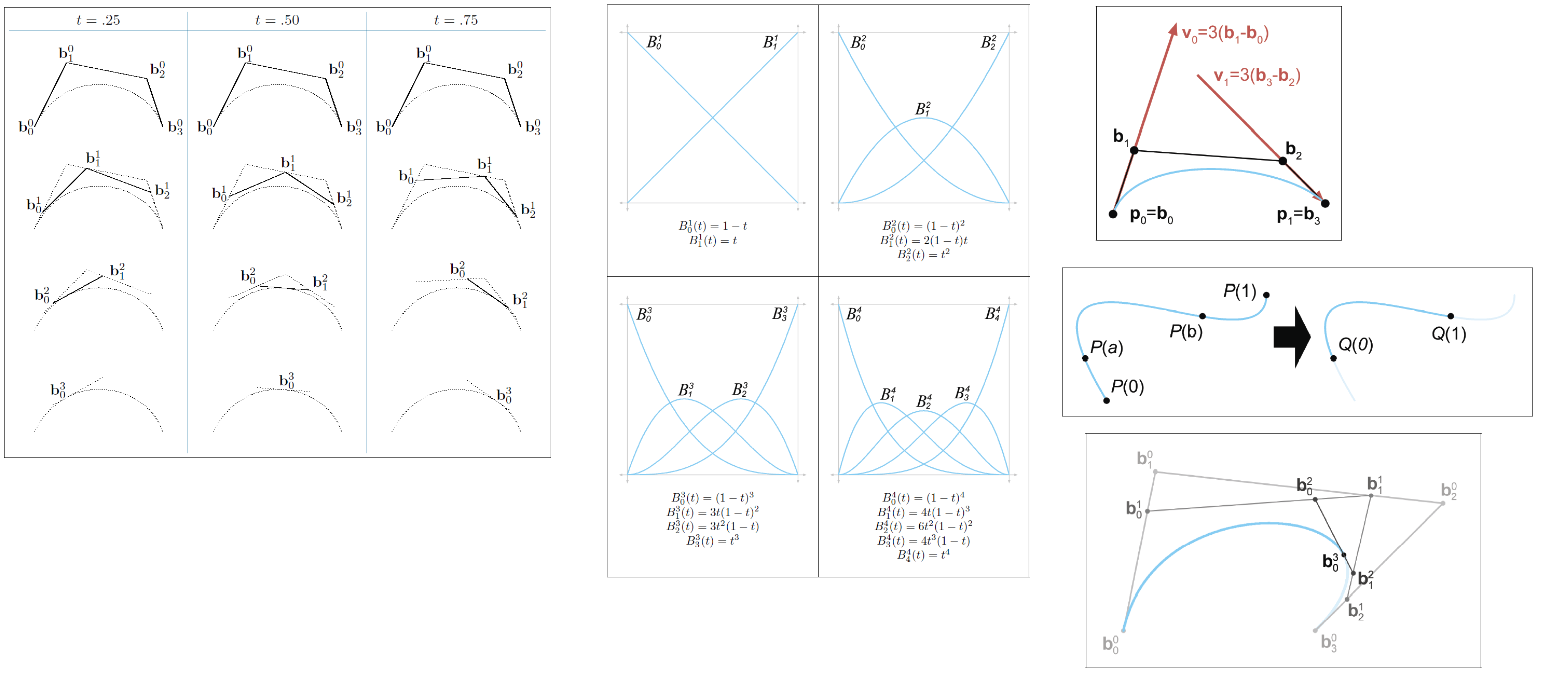
The de Casteljau Algorithm
The de Casteljau algorithm defines a method for constructing B´ezier curves through repeated linear interpolation.
De Casteljau Recurrence Relation
$$
b_i^0(t) = b_i\\
b_i^n(t) = (1-t)[b_i^{n-1}(t)] + t[b_{i+1}^{n-1}(t)]
$$
The cubic equation for a specific point on the curve $p(t)$ is written in matrix notation as
$$
\begin{aligned}
\vec{p(t)} &= C\vec{t}\\
&= \begin{bmatrix}
\vec{c_0} &\vec{c_1} & \vec{c_2} & \vec{c_3}
\end{bmatrix}
\begin{bmatrix}
1 \\ t \\ t^2 \\ t^3
\end{bmatrix}\\
&= BM\vec{t}\\
&=
\begin{bmatrix}
\vec{b_0} &\vec{b_1} & \vec{b_2} & \vec{b_3}
\end{bmatrix}
\begin{bmatrix}
1 & -3 & 3 & 1\\
0 & 3 & -6 & 3\\
0 & 0 & -3 & -3\\
0 & 0 & 0 & 1
\end{bmatrix}
\begin{bmatrix}
1 \\ t \\ t^2 \\ t^3
\end{bmatrix}
\end{aligned}
$$
The Bernstein Basis
We can also write the polynomial in B´ezier form by collecting the terms on the control points rather than the powers of $t$. When written this way, each control point has a coefficient that represents the barycentric weight as a function of $t$ that the control point contributes to the curve.
Now that we get:
$$
\begin{aligned}
b_0^1(t) &= (1-t)b_0 + tb_1\\
b_0^2(t) &= (1-t)^2b_0 + 2t(1-t)b_1 + t^2b_2\\
b_0^3(t) &= (1-t)^3b_0 + 3t(1-t)^2b_1 + 3t^2(1-t)b_2 + t^3b_3\\
\cdots
\end{aligned}
$$
Thus, we can see the pattern:
$$
\begin{aligned}
b_0^n(t) &= \sum_{i=0}^n[B_i^n(t)]b_i\\
B_i^n(t) &= \begin{pmatrix}n \\ i\end{pmatrix}t^i(1-t)^{n-i}, 0 \leq i \leq n\\
\begin{pmatrix}n \\ i\end{pmatrix} &= \frac{n!}{k!(n-k)!}
\end{aligned}
$$
The properties of the Bernstein polynomials tell us a lot about how B´ezier curves behave.
Sum to one.
The Bernstein polynomials sum to unity for all values of $t$, which is nice because if they didn’t, then they wouldn’t define proper barycentric coordinates.
Convex hull property.
The range of the Bernstein polynomials is $0 \cdots 1$ for the entire length of the curve, $0 ≤ t ≤ 1$. The curve is bounded to stay within the convex hull of the control points.Endpoints interpolated.
Global support.
The practical result is that when any one control point is moved, the entire curve is affected. This is not a desirable property for curve design.One local maximum.
Each Bernstein polynomial $B_i^n(t)$, which serves as the blend weight for the control point $b_i$, has one maximum at the auspicious time $t = i/n$.
B´ezier Derivatives and Their Relationship to the Hermite Form
The $nth$ derivative at either endpoint is completely determined by the nearest $n + 1$ control points.
The second derivative (acceleration) at the end of the curve is determined by the closest three control points.
Subdivision
Why need subdivision?
- Curve refinement.
- Approximation techniques.
Subdividing Curves in Monomial Form
the problem of subdivision can easily be viewed as a simple problem of reparameterization.
$$
t = F(s)\\
q(s) = p(t) = p(F(s))
$$
$$
\begin{cases}
F(0) = a\\
F(1) = b
\end{cases}
\longmapsto
t = F(s) = a + s(b-a), s \in [0,1]
$$
Subdividing Curves in B´ezier Form
As it turns out, each round of de Casteljau interpolation produces one of our B´ezier control points.
Thus,
To extract the left half of a curve, $0 ≤ t ≤ b$, we perform de Casteljau subdivision as if we were trying to locate the endpoint at $t = b$. The first control point from each round of interpolation gives us another control point for our subdivided curve.
Spline
Rules of the Game
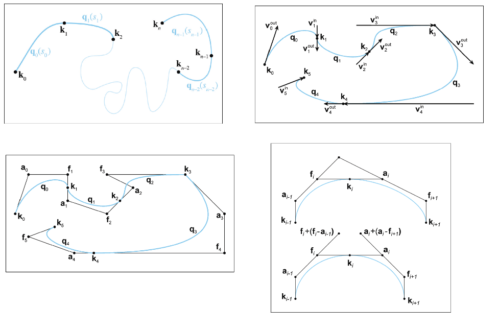
the function $q(s)$ refers to the entire spline, and the parameter $s$ (without subscript) is a global parameter. As $s$ varies from $0$ to $n$, the function $q(s)$ traces out the entire spline.
In general, we can define $p(t)$ in terms of $q(s)$ by creating a function that maps a time value $t$ to a parameter value $s$.
If you’re a computer programmer, you can think of $p(t)$ as the public interface, and $q(s)$ as an internal implementation detail.
Map the time value $t$ into a value of $s$ by evaluating the time-toparameter function $s(t)$.
Extract the integer portion of $s$ as $i$, and the fractional portion as $s_i$.
Evaluate the curve segment $q_i(s_i)$.
Knots
For the curve to be continuous, clearly the ending point of one segment must be coincident with the starting point of the next segment. These shared control points that are interpolated by the spline are called the knots of the spline.
In animation contexts, the knots are sometimes called keys. In computer animation, a key can be any position, orientation, or other piece of data whose value at a particular time is specified by a human animator (or any other source). The role of the apprentice to “fill in the missing frames” is played by the animation program, using interpolation methods such as the ones being discussed in this chapter.
Hermite and B´ezier Splines
When we were focused on a single segment, we denoted the positions by $p_0$ and $p_1$, and the velocities(tangents) by $v_0$ and $v_1$.
the knot $k_i$, which is the starting position of the segment $q_i(0)$, also serves as the ending position of the previous segment at $q_{i−1}(1)$. For velocities, the notation $v^{out}_i$ refers to the outgoing velocity at knot $i$ and defines the starting velocity for the segment $q_i$.
(Photoshop calls the knots the “anchor points” and refers to the interior B´ezier control points that are not interpolated as “control points.”)
When we were dealing with only a single B´ezier segment, we referred to the $ith$ control point on that segment as $b_i$. Here we use the notation $f_i$ to refer to the control point “in front” of the ith knot, and $a_i$ for the control point “after” it.
Converting between B´ezier and Hermite forms:
$$
\begin{aligned}
&v_i^{in} = 3(k_i - f_i), f_i = k_i - v_i^{in}/3\\
&v_i^{out} = 3(a_i - k_i), a_i = k_i + v_i^{out}/3
\end{aligned}
$$
Continuity
Parametric Continuity
A curve is said to have $C^n$ continuity if its first $n$ derivatives are continuous.
$C^1$ continuity condition for Hermite splines:
$$
v_i^{in} = v_i^{out}
$$
$C^1$ continuity condition for cubic B´ezier splines
$$
k_i - f_i = a_i - k_i
$$
$C^2$ continuity condition for cubic B´ezier splines
$$
f_i + (f_i - a_{i-1}) = a_i + (a_i - f_{i+1})
$$
Geometric Continuity
$G^1$: the tangents are parallel at the knot. if the tangents are parallel, then the discontinuity is purely a change in speed, not a change in direction.
We say that a curve is $G^2$ continuous if its curvature changes continuously.
Automatic Tagent Control
We want to get the smooth curve only by several knots, without the need for the user to specify any additional criteria(like the $C^1$ continuity).
CatmullRom Splines
the formular of Catmull-Rom Spline
$$
\begin{aligned}
v_i^{in} &= v_i^{out} = \frac{k_{i+1} - k_{i-1}}{2}\\
&=\frac{(k_{i+1} - k_i) + (k_i - k_{i-1})}{2}
\end{aligned}
$$