Calculus-C14-Partial-Derivatives

Keywords: Partial Derivatives, Directional Derivatives and Gradient Vectors, Lagrange Multipliers

This is the Chapter14 ReadingNotes from book Thomas Calculus 14th.

Functions of Several Variables

DEFINITIONS
Suppose $D$ is a set of $n$-tuples of real numbers $(x_1, x_2, \cdots , x_n)$. A real-valued function $ƒ$ on $D$ is a rule that assigns a unique (single) real number
$$
w = f(x_1, x_2, \cdots , x_n)
$$
to each element in $D$. The set $D$ is the function’s domain. The set of $w$-values taken on by $ƒ$ is the function’s range. The symbol $w$ is the dependent variable of $ƒ$, and $ƒ$ is said to be a function of the $n$ independent variables $x_1$ to $x_n$. We also call the $x_j$’s the function’s input variables and call $w$ the function’s output variable.

Domains and Ranges

The domain of a function is assumed to be the largest set for which the defining rule generates real numbers, unless the domain is otherwise specified explicitly. The range consists of the set of output values for the dependent variable.

Functions of Two Variables

DEFINITIONS
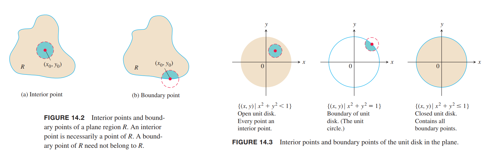
A point $(x_0, y_0)$ in a region (set) $R$ in the $xy$-plane is an interior point of $R$ if it is the center of a disk of positive radius that lies entirely in R (Figure 14.2). A point $(x_0, y_0)$ is a boundary point of $R$ if every disk centered at $(x_0, y_0)$ contains points that lie outside of $R$ as well as points that lie in $R$. (The boundary point itself need not belong to $R$.)
The interior points of a region, as a set, make up the interior of the region. The region’s boundary points make up its boundary. A region is open if it consists entirely of interior points. A region is closed if it contains all its boundary points (Figure 14.3).

DEFINITIONS
A region in the plane is bounded if it lies inside a disk of finite radius. A region is unbounded if it is not bounded.

Graphs, Level Curves, and Contours of Functions of Two Variables

DEFINITIONS
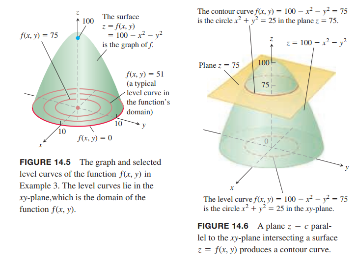
The set of points in the plane where a function $ƒ(x, y)$ has a constant value $ƒ(x, y) = c$ is called a level curve（等高线） of $ƒ$. The set of all points $(x, y, ƒ(x, y))$ in space, for $(x, y)$ in the domain of $ƒ$, is called the graph of $ƒ$. The graph of $ƒ$ is also called the surface $z = ƒ(x, y)$.

Functions of Three Variables

DEFINITION
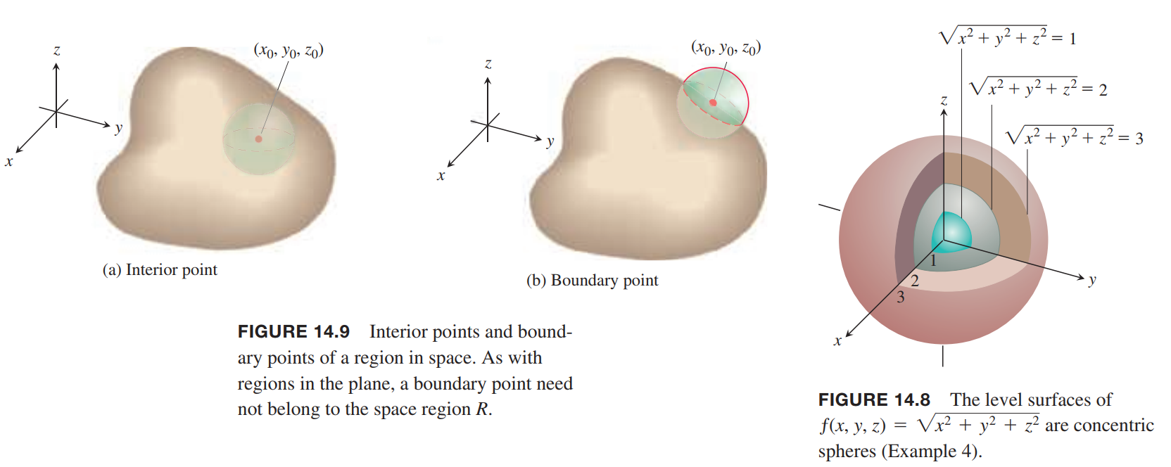
The set of points $(x, y, z)$ in space where a function of three independent variables has a constant value $ƒ(x, y, z) = c$ is called a level surface of $ƒ$.

Since the graphs of functions of three variables consist of points $(x, y, z, ƒ(x, y, z))$ lying in a four-dimensional space, we cannot sketch them effectively in our three-dimensional frame of reference. We can see how the function behaves, however, by looking at its three-dimensional level surfaces.

DEFINITIONS
A point $(x_0, y_0, z_0)$ in a region $R$ in space is an interior point of $R$ if it is the center of a solid ball that lies entirely in $R$ (Figure 14.9a). A point $(x_0, y_0, z_0)$ is a boundary point of $R$ if every solid ball centered at $(x_0, y_0, z_0)$ contains points that lie outside of $R$ as well as points that lie inside R (Figure 14.9b). The interior of $R$ is the set of interior points of $R$. The boundary of $R$ is the set of boundary points of $R$.
A region is open if it consists entirely of interior points. A region is closed if it contains its entire boundary.

Computer Graphing

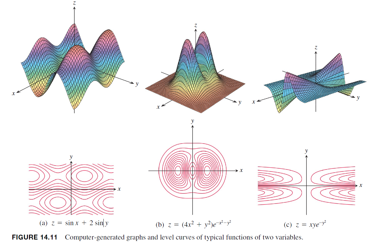
Figure 14.11 shows computer-generated graphs of a number of functions of two variables together with their level curves.

Limits and Continuity in Higher Dimensions

Limits for Functions of Two Variables

Definition
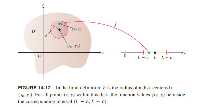
We say that a function ƒ(x, y) approaches the limit $L$ as $(x, y)$ approaches $(x_0 , y_0)$, and write
$$
\lim_{(x,y)\rightarrow (x_0,y_0)} f(x,y) = L
$$
if, for every number $\epsilon > 0$, there exists a corresponding number $\delta > 0$ such that for all $(x, y)$ in the domain of $ƒ$,
$$
|f(x,y) - L| < \epsilon, whenever, 0 < \sqrt{(x-x_0)^2 + (y-y_0)^2} < \delta
$$

Continuity

Definition
A function ƒ(x, y) is continuous at the point $(x_0 , y_0)$ if

1. ƒ is defined at $(x_0 , y_0)$,
2. $\lim_{(x, y)\rightarrow (x_0, y_0)} ƒ(x, y)$ exists,
3. $\lim_{(x, y)\rightarrow (x_0, y_0)} ƒ(x, y) = f(x_0,y_0)$.
   A function is continuous if it is continuous at every point of its domain.

Continuity of Compositions
If $ƒ$ is continuous at $(x_0 , y_0)$ and $g$ is a single-variable function continuous at $ƒ(x_0 , y_0)$, then the composition $h = g \circ f$ defined by $h(x, y) = g(ƒ(x, y))$ is continuous at $(x_0, y_0)$.

Partial Derivatives

Partial Derivatives of a Function of Two Variables

DEFINITION
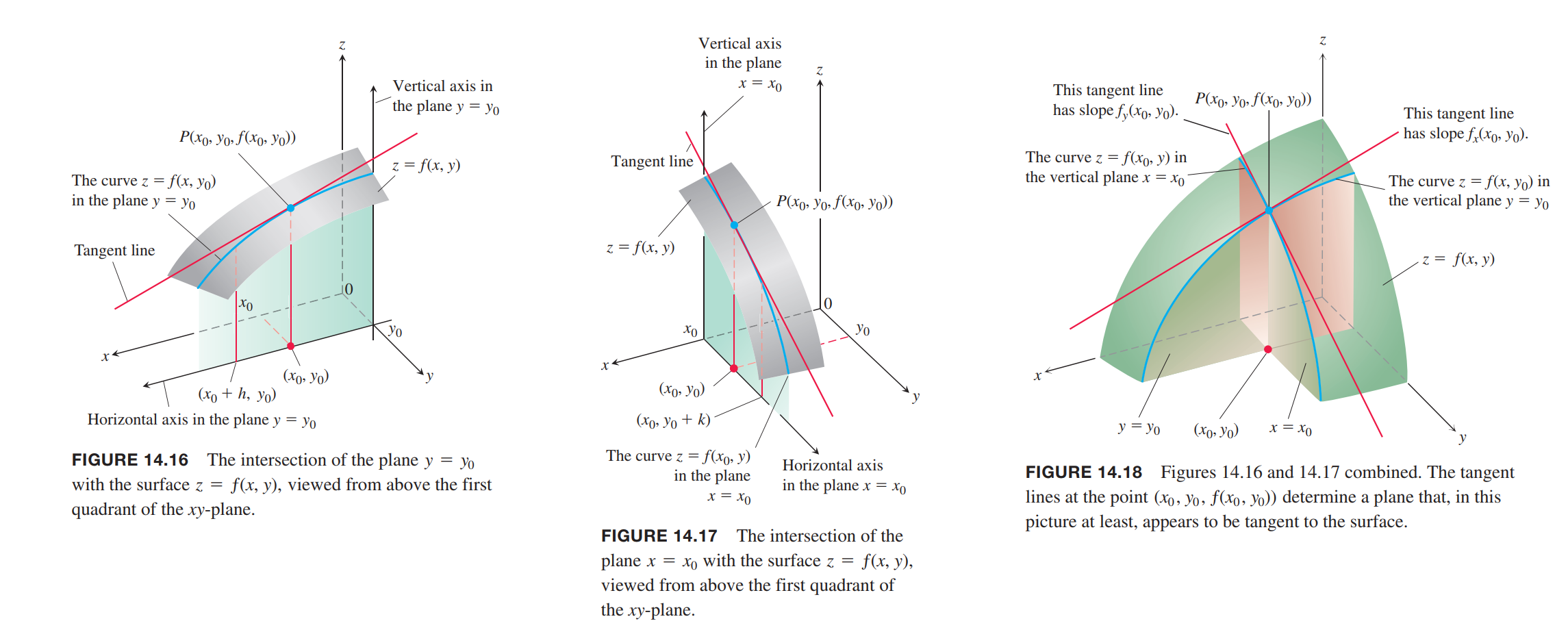
The partial derivative of $ƒ(x, y)$ with respect to $x$ at the point $(x_0 , y_0)$ is
$$
\left. \frac{\partial f}{\partial x} \right|_{x_0, y_0} = \lim_{h\rightarrow 0} \frac{f(x_0+h,y_0) - f(x_0,y_0)}{h}
$$
The partial derivative of $ƒ(x, y)$ with respect to $y$ at the point $(x_0 , y_0)$ is
$$
\left. \frac{\partial f}{\partial y} \right|_{x_0, y_0} = \lim_{h\rightarrow 0} \frac{f(x_0,y_0 + h) - f(x_0,y_0)}{h}
$$

Calculations

💡For example💡:

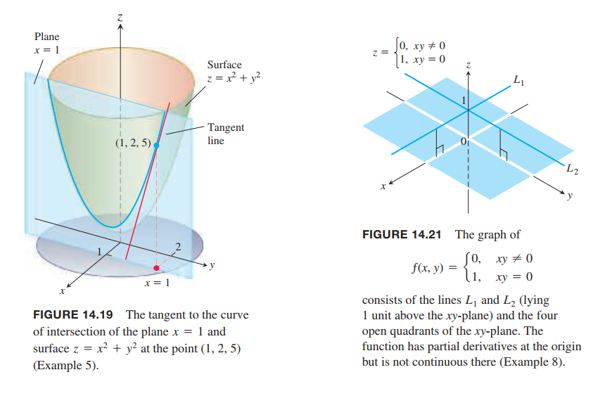
The plane $x = 1$ intersects the paraboloid（抛物面） $z = x^2 + y^2$ in a parabola（抛物线）. Find the slope of the tangent to the parabola at $(1, 2, 5)$ (Figure 14.19).

Solution:

The parabola lies in a plane parallel to the $yz$-plane, and the slope is the value of the partial derivative $\frac{\partial z}{\partial y}$ at $(1, 2)$:

$$
\left. \frac{\partial z}{\partial y} \right|_{(1,2)} = \left. 2y \right|_{(1,2)} = 4
$$

Functions of More Than Two Variables

Partial Derivatives and Continuity

A function $ƒ(x, y)$ can have partial derivatives with respect to both $x$ and $y$ at a point without the function being continuous there.（对于多变量（元）函数，偏导存在(可导)不一定连续）

💡For example💡:

Let
$$
f(x,y) =
\begin{cases}
0, xy \neq 0\\
1, xy = 0
\end{cases}
$$
(Figure 14.21).
(a) Find the limit of $ƒ$ as $(x, y)$ approaches $(0, 0)$ along the line $y = x$.
(b) Prove that $ƒ$ is not continuous at the origin.
(c) Show that both partial derivatives $\partial ƒ /\partial x$ and $\partial ƒ /\partial y$ exist at the origin.

Solution:

(a). Since $ƒ(x, y)$ is constantly zero along the line $y = x$ (except at the origin), we have

$$
\left. \lim_{(x,y) \rightarrow (0,0)} f(x,y) \right|_{y=x} = \lim_{(x,y) \rightarrow (0,0)} 0 = 0
$$

(b). Since $ƒ(0, 0) = 1$, the limit in part (a) is not equal to $ƒ(0, 0)$, which proves that $ƒ$ is not continuous at $(0, 0)$.

(c). To find $\partial ƒ /\partial x$ at $(0, 0)$, we hold $y$ fixed at $y = 0$. Then $ƒ(x, y) = 1$ for all $x$, and the graph of $ƒ$ is the line $L1$ in Figure 14.21. The slope of this line at any $x$ is $\partial ƒ /\partial x$. In particular, $\partial ƒ /\partial x = 0$ at $(0, 0)$. Similarly, $\partial ƒ /\partial y$ is the slope of line $L2$ at any $y$, so $\partial ƒ /\partial y = 0$ at $(0, 0)$.

Second-Order Partial Derivatives

$$
\frac{\partial f}{\partial x \partial y}
\Longleftrightarrow
f_{yx}
$$
Differentiate first with respect to $y$, then with respect to $x$.

The Mixed Derivative Theorem

THEOREM 2—The Mixed Derivative Theorem
If $ƒ(x, y)$ and its partial derivatives $f_x, f_y, f_{xy}, f_{yx}$ are defined throughout an open region containing a point $(a, b)$ and are all continuous at $(a, b)$, then
$$
f_{xy}(a,b) = f_{yx}(a,b)
$$

Partial Derivatives of Still Higher Order

Differentiability

DEFINITION
A function $z = ƒ(x, y)$ is differentiable at $(x_0, y_0)$ if $ƒ_x(x_0 , y_0)$ and $ƒ_y(x_0, y_0)$ exist and $\Delta z = ƒ(x_0 + \Delta x, y_0 + \Delta y) - ƒ(x_0, y_0)$ satisfies an equation of the form
$$
\Delta z = f_x(x_0, y_0) \Delta x + f_y(x_0,y_0)\Delta y + \epsilon_1 \Delta x + \epsilon_2 \Delta y
$$
in which each of $\epsilon_1, \epsilon_2 \rightarrow 0$ as both $\Delta x, \Delta y \rightarrow 0$. We call $ƒ$ differentiable if it is differentiable at every point in its domain, and say that its graph is a smooth surface.

THEOREM 4—Differentiability Implies Continuity（对于多变量（元）函数，可微一定连续）
If a function $ƒ(x, y)$ is differentiable at $(x_0 , y_0)$, then $ƒ$ is continuous at $(x_0 , y_0)$.

👉More about Derivative and Differentiation in Single Variable Function

The Chain Rule

Functions of Two Variables

Theorem 5—Chain Rule For Functions of One Independent Variable and Two Intermediate Variables
If $w = ƒ(x, y)$ is differentiable and if $x = x(t), y = y(t)$ are differentiable functions of $t$, then the composition $w = ƒ(x(t), y(t))$ is a differentiable function of $t$ and
$$
\frac{dw}{dt} = f_x(x(t), y(t)) x’(t) + f_y(x(t), y(t)) y’(t)
$$
or
$$
\frac{dw}{dt} = \frac{\partial f}{\partial x} \frac{dx}{dt} + \frac{\partial f}{\partial y} \frac{dy}{dt}
$$

Functions of Three Variables

Theorem 6—Chain Rule for Functions of One Independent Variable and Three Intermediate Variables
If $w = ƒ(x, y, z)$ is differentiable and $x, y$, and $z$ are differentiable functions of $t$, then $w$ is a differentiable function of $t$ and
$$
\frac{dw}{dt} = \frac{\partial w}{\partial x} \frac{dx}{dt} + \frac{\partial w}{\partial y} \frac{dy}{dt} + + \frac{\partial w}{\partial z} \frac{dz}{dt}
$$

Functions Defined on Surfaces

THEOREM 7—Chain Rule for Two Independent Variables and Three Intermediate Variables
Suppose that $w = ƒ(x, y, z)$, $x = g(r, s), y = h(r, s)$, and $z = k(r, s)$. If all four functions are differentiable, then $w$ has partial derivatives with respect to $r$ and $s$, given by the formulas
$$
\frac{\partial w}{\partial r} = \frac{\partial w}{\partial x}\frac{\partial x}{\partial r} + \frac{\partial w}{\partial y}\frac{\partial y}{\partial r} + \frac{\partial w}{\partial z}\frac{\partial z}{\partial r}
$$
$$
\frac{\partial w}{\partial s} = \frac{\partial w}{\partial x}\frac{\partial x}{\partial s} + \frac{\partial w}{\partial y}\frac{\partial y}{\partial s} + \frac{\partial w}{\partial z}\frac{\partial z}{\partial s}
$$

Implicit Differentiation Revisited

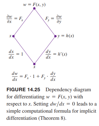
Suppose that

1. The function $F(x, y)$ is differentiable and
2. The equation $F(x, y) = 0$ defines $y$ implicitly as a differentiable function of $x$, say $y = h(x)$.

Since $w = F(x, y) = 0$, the derivative $dw/ dx$ must be zero.

$$
0 = \frac{dw}{dx} = F_x\frac{dx}{dx} + F_y\frac{dy}{dx}
= F_x \cdot 1 + F_y \cdot \frac{dy}{dx}
$$

If $F_y = \frac{\partial w}{\partial y} \neq 0$, then

$$
\frac{dy}{dx} = -\frac{F_x}{F_y}
$$

Functions of Many Variables

Directional Derivatives and Gradient Vectors

Directional Derivatives in the Plane

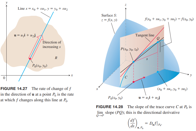
Suppose that the function $ƒ(x, y)$ is defined throughout a region $R$ in the $xy$-plane, that $P_0(x_0, y_0)$ is a point in $R$, and that $\vec{u} = u_1\vec{i} + u_2\vec{j}$ is a unit vector. Then the equations
$$
x = x_0 + s\vec{u_1}, y = y_0 + s\vec{u_2}
$$
parametrize the line through $P_0$ parallel to $\vec{u}$.

If the parameter $s$ measures arc length from $P_0$ in the direction of $\vec{u}$, we find the rate of change of $ƒ$ at $P_0$ in the direction of $\vec{u}$ by calculating $dƒ / ds$ at $P_0$.

DEFINITION
The derivative of $f$ at $P_0(x_0, y_0)$ in the direction of the unit vector $\vec{u} = u_1\vec{i} + u_2\vec{j}$ is the number
$$
\left( \frac{df}{ds} \right)_{\vec{u}, P_0} = \lim_{s \rightarrow 0} \frac{f(x_0 + su_1, y_0 + su_2) - f(x_0,y_0)}{s}
\tag{1}
$$
The directional derivative defined by Equation (1) is also denoted by
$$
D_{\vec{u}} f(P_0)\\
or\\
\left. D_{\vec{u}} f \right|_{P_0}
$$

Interpretation of the Directional Derivative

The equation $z = ƒ(x, y)$ represents a surface $S$ in space. If $z_0 = ƒ(x_0 , y_0)$, then the point $P(x_0 , y_0 , z_0)$ lies on $S$. The vertical plane that passes through $P$ and $P_0(x_0 , y_0)$ parallel to $\vec{u}$ intersects $S$ in a curve $C$ (Figure 14.28). The rate of change of $ƒ$ in the direction of $\vec{u}$ is the slope of the tangent to $C$ at $P$ in the right-handed system formed by the vectors $\vec{u}$ and $\vec{k}$.

Calculation and Gradients

By Chain Rule:

$$
\begin{aligned}
\left( \frac{df}{ds}\right)_{\vec{u},P_0} &= \left. \frac{\partial f}{\partial x} \right|_{P_0} \frac{dx}{ds} + \left. \frac{\partial f}{\partial y} \right|_{P_0} \frac{dy}{ds}\\
&= \left. \frac{\partial f}{\partial x} \right|_{P_0} u_1 + \left. \frac{\partial f}{\partial x} \right|_{P_0} u_2 \\
&= \underbrace{\left[ \left. \frac{\partial f}{\partial x} \right|_{P_0} \vec{i} + \left. \frac{\partial f}{\partial y} \right|_{P_0} \vec{j} \right]}_{Gradient-of-f-at-P_0} \cdot \underbrace{\left[ u_1\vec{i} + u_2\vec{j} \right]}_{Direction-of-\vec{u}}
\end{aligned}
\tag{3}
$$

Definition
The gradient vector (or gradient) of $ƒ(x, y)$ is the vector
$$
\nabla f = \frac{\partial f}{\partial x} \vec{i} + \frac{\partial f}{\partial y} \vec{j}
$$
The value of the gradient vector obtained by evaluating the partial derivatives at a point $P_0(x_0, y_0)$ is written
$$
\left. \nabla f \right|_{P_0}\\
or\\
\nabla f(x_0,y_0)
$$

theorem 9—The Directional Derivative Is a Dot Product
If $ƒ(x, y)$ is differentiable in an open region containing $P_0(x_0, y_0)$, then
$$
\left( \frac{df}{ds} \right)_{\vec{u}, P_0} = \left. \nabla f \right|_{P_0} \cdot \vec{u}
\tag{4}
$$

💡For example💡:

Find the derivative of $ƒ(x, y) = xe^y + cos (xy)$ at the point $(2, 0)$ in the direction of $\vec{v} = 3\vec{i} - 4\vec{j}$.（directional derivative）

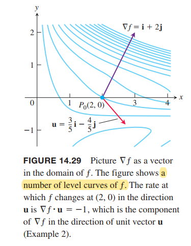
Solution:

Recall that the direction of a vector $\vec{v}$ is the unit vector obtained by dividing $\vec{v}$ by its length:

$$
\vec{u} = \frac{\vec{v}}{|\vec{v}|} = \frac{3}{5}\vec{i} - \frac{4}{5}\vec{j}
$$

The partial derivatives of $f$ are everywhere continuous and at $(2, 0)$ are given by

$$
f_x(2,0) = \left. (e^y - y\sin(xy)) \right|_{(2,0)} = 1\\
f_y(2,0) = 2
$$

The gradient of $ƒ$ at $(2, 0)$ is

$$
\left. \nabla f \right|_{2,0} = f_x(2,0) \vec{i} + f_y(2,0)\vec{j} = \vec{i} + 2\vec{j}
$$

The derivative of $f$ at $(2, 0)$ in the direction of $\vec{v}$ is therefore

$$
D_{\vec{u}} f |_{(2,0)} = \nabla f_{(2,0)} \cdot \vec{u}
= -1
$$

Evaluating the dot product in the brief version of Equation (4) gives
$$
D_{\vec{u}} f = \nabla f \cdot \vec{u} = |\nabla f| |\vec{u}| \cos \theta = |\nabla f| \cos \theta
$$

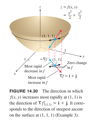
Properties of the Directional Derivative $D_{\vec{u}} f = \nabla f \cdot \vec{u} = |\nabla f| \cos \theta$

1. The function $ƒ$ increases most rapidly when $\cos\theta = 1$, which means that $\theta = 0$ and $\vec{u}$ is the direction of $\nabla f$. That is, at each point $P$ in its domain, $ƒ$ increases most rapidly in the direction of the gradient vector $\nabla f$ at $P$. The derivative in this direction is
   $$
   D_{\vec{u}} f = |\nabla f| \cos(0) = |\nabla f|
   $$
2. Similarly, $ƒ$ decreases most rapidly in the direction of $-\nabla f$. The derivative in this direction is $D_{\vec{u}} f = |\nabla f| \cos(\pi) = -|\nabla f|$.
3. Any direction $\vec{u}$ orthogonal to a gradient $\nabla f \neq 0$ is a direction of zero change in $ƒ$ because $\theta$ then equals $\pi / 2$ and
   $$
   D_{\vec{u}} f = |\nabla f| \cos(\pi/2) = 0
   $$

Gradients and Tangents to Level Curves

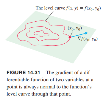
If a differentiable function $ƒ(x, y)$ has a constant value $c$ along a smooth curve $r = g(t)i + h(t)j$, then
$$
\frac{d}{dt}f(g(t), h(t)) = \frac{d}{dt} c
$$

$$
\frac{\partial f}{\partial x}\frac{dg}{dt} + \frac{\partial f}{\partial y}\frac{dh}{dt} = 0
$$

$$
\underbrace{\left( \frac{\partial f}{\partial x} \vec{i} + \frac{\partial f}{\partial y} \vec{j}\right)}_{\nabla f} \cdot
\underbrace{\left( \frac{dg}{dt} \vec{i} + \frac{dh}{dt} \vec{j}\right)}_{\frac{dr}{dt}} = 0
\tag{5}
$$
Equation (5) says that $\nabla ƒ$ is normal to the tangent vector $dr / dt$, so it is normal to the curve.

Tangent Line to a Level Curve
$$
f_x(x_0,y_0)(x-x_0) + f_y(x_0,y_0)(y-y_0) = 0
$$

Attention：gradient is perpendicular to the level curve, not the surface. Gradient in multi-variable function is like derivative in sigle-variable function.

Functions of Three Variables

The Chain Rule for Paths

If $r(t) = x(t) i + y(t) j + z(t)k$ is a smooth path $C$, and $w = ƒ(r(t))$ is a scalar function evaluated along $C$, then according to the Chain Rule,
$$
\frac{dw}{dt} = \frac{\partial w}{\partial x} \frac{dx}{dt} + \frac{\partial w}{\partial y} \frac{dy}{dt} + \frac{\partial w}{\partial z} \frac{dz}{dt}
$$

The Derivative Along a Path
$$
\frac{d}{dt}f(r(t)) = \nabla f(r(t)) \cdot r’(t)
\tag{7}
$$
What Equation (7) says is that the derivative of the composite function $ƒ(r(t))$ is the “derivative” (gradient) of the outside function $ƒ$ “times” (dot product) the derivative of the inside function $r$.

Tangent Planes and Differentials

Recall how the derivative defined the tangent line to the graph of a differentiable function at a point on the graph. The tangent line then provided for a linearization of the function at the point. 👉More about Tangent Line in Singule Variable Function >>

how the gradient defines the tangent plane to the level surface of a function $w = ƒ(x, y, z)$ at a point on the surface. The tangent plane then provides for a linearization of $ƒ$ at the point and defines the total differential of the function.

Tangent Planes and Normal Lines

DEFINITIONS
The tangent plane to the level surface $ƒ(x, y, z) = c$ of a differentiable function $ƒ$ at a point $P_0$ where the gradient is not zero is the plane through $P_0$ normal to $\nabla f|_{P_0}$.
The normal line of the surface at $P_0$ is the line through $P_0$ parallel to $\nabla f |_{P_0}$.

💡For example💡:

Find the tangent plane and normal line of the level surface
$$
f(x,y,z) = x^2 + y^2 + z - 9 = 0
$$
at the point $P_0 (1, 2, 4)$.

Solution:

The tangent plane is the plane through $P_0$ perpendicular to the gradient of $ƒ$ at $P_0$. The gradient is
$$
\nabla f |_{P_0} = (2xi + 2yj + k)|_{(1,2,4)} = 2i + j + k
$$
The tangent plane is therefore the plane
$$
2(x-1) + 4(y-2) + (z-4) = 0
$$
or
$$
2x + 4y + z = 14
$$
The line normal to the surface at $P_0$ is
$$
x = 1 + 2t, y = 2 + 4t, z = 4 + t
$$

Plane Tangent to a Surface $z = ƒ(x, y)$ at $(x_0 , y_0 , ƒ(x_0 , y_0))$
The plane tangent to the surface $z = ƒ(x, y)$ of a differentiable function $ƒ$ at the point $P_0(x_0 , y_0 , z_0) = (x_0 , y_0 , ƒ(x_0 , y_0))$ is
$$
f_x(x_0,y_0)(x-x_0) + f_y(x_0,y_0)(y-y_0)-(z-z_0) = 0
$$

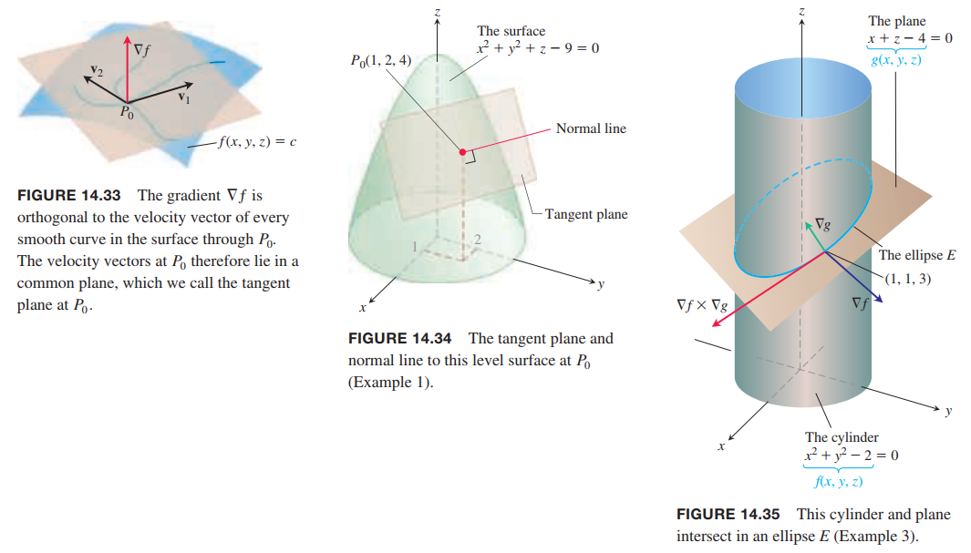
💡For example💡:

The surfaces

$$
f(x,y,z) = x^2 + y^2 -2 = 0
$$
and

$$
g(x,y,z) = x + z - 4 = 0
$$

meet in an ellipse $E$ (Figure 14.35). Find parametric equations for the line tangent to $E$ at the point $P_0(1, 1, 3)$.

Solution:

The tangent line is orthogonal to both $\nabla f$ and $\nabla g$ at $P_0$, and therefore parallel to $v = \nabla f \times \nabla g$. The components of $v$ and the coordinates of $P_0$ give us equations for the line. We have

$$
\nabla f |_{(1,1,3)} = 2i + 2j
$$

$$
\nabla g |_{(1,1,3)} = i + k
$$

$$
\begin{aligned}
v &= (2i + 2j) \times (i + k)\\
&=
\begin{vmatrix}
i & j & k \\
2 & 2 & 0\\
1 & 0 & 1
\end{vmatrix}\\
&=2i - 2j - 2k
\end{aligned}
$$

The tangent line to the ellipse of intersection is
$$
x = 1 + 2t, y = 1 - 2t, z = 3 - 2t
$$

Estimating Change in a Specific Direction

Estimating the Change in $ƒ$ in a Direction $u$
To estimate the change in the value of a differentiable function $ƒ$ when we move a small distance $ds$ from a point $P_0$ in a particular direction $u$, use the formula
$$
df = \underbrace{(\nabla f |_{P_0} \cdot u)}_{Directional-derivative} \underbrace{ds}_{Distance-increment}
$$

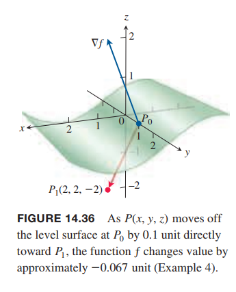
💡For example💡:

Estimate how much the value of

$$
f(x,y,z) = y\sin x + 2yz
$$
will change if the point $P(x, y, z)$ moves $0.1$ unit from $P_0(0, 1, 0)$ straight toward $P_1(2, 2, -2)$.

Solution:

We first find the derivative of $ƒ$ at $P_0$ in the direction of the vector $\vec{P_0P_1} = 2i + j - 2k$. The direction of this vector is
$$
u = \frac{\vec{P_0P_1}}{|\vec{P_0P_1}|} = \frac{2}{3}i + \frac{1}{3}j - \frac{2}{3}k
$$
The gradient of $ƒ$ at $P_0$ is
$$
\nabla f|_{(0,1,0)} = i + 2k
$$
Therefore,
$$
\nabla f|_{P_0} \cdot u = -\frac{2}{3}
$$
The change $dƒ$ in $ƒ$ that results from moving $ds = 0.1$ unit away from $P_0$ in the direction of $u$ is approximately
$$
df = (\nabla f|_{P_0} \cdot u)(ds) \approx -0.047unit.
$$

How to Linearize a Function of Two Variables

DEFINITIONS
The linearization of a function $ƒ(x, y)$ at a point $(x_0 , y_0)$ where $ƒ$ is differentiable is the function
$$
L(x,y) = f(x_0,y_0) + f_x(x_0,y_0)(x-x_0) + f_y(x_0,y_0)(y-y_0)
$$
The approximation
$$
f(x,y) \approx L(x,y)
$$
is the standard linear approximation of $ƒ$ at $(x_0 , y_0)$.

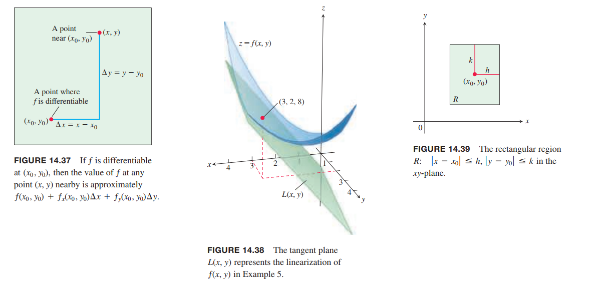
Thus, the linearization of a function of two variables is a tangent-plane approximation in the same way that the linearization of a function of a single variable is a tangent-line approximation.

The Error in the Standard Linear Approximation
If $ƒ$ has continuous first and second partial derivatives throughout an open set containing a rectangle $R$ centered at $(x_0, y_0)$ and if $M$ is any upper bound for the values of $|f_{xx}|,|f_{yy}|$, and $|f_{xy}|$ on $R$, then the error $E(x, y)$ incurred in replacing $ƒ(x, y)$ on $R$ by its linearization
$$
L(x,y) = f(x_0, y_0) + f_x(x_0,y_0)(x-x_0) + f_y(x_0,y_0)(y-y_0)
$$
satisfies the inequality
$$
|E(x,y)| \leq \frac{1}{2}M(|x-x_0| + |y-y_0|)^2
$$

Differentials

Definition
If we move from $(x_0, y_0)$ to a point $(x_0 + dx, y_0 + dy)$ nearby, the resulting change
$$
df = f_x(x_0,y_0)dx + f_y(x_0,y_0)dy
$$
in the linearization of $ƒ$ is called the total differential of $ƒ$.

Functions of More Than Two Variables

The linearization of $ƒ(x, y, z)$ at a point $P_0(x_0, y_0, z_0)$ is
$$
L(x,y,z) = f(P_0) + f_x(P_0)(x-x_0) + f_y(P_0)(y-y_0) + f_z(P_0)(z-z_0)
$$

Extreme Values and Saddle Points

👉Similar Meanings in Single-Variable Functions

Derivative Tests for Local Extreme Values

DEFINITIONS
Let $ƒ(x, y)$ be defined on a region $R$ containing the point $(a, b)$. Then

1. $ƒ(a, b)$ is a local maximum value of $ƒ$ if $ƒ(a, b) \geq ƒ(x, y)$ for all domain points $(x, y)$ in an open disk centered at $(a, b)$.
2. $ƒ(a, b)$ is a local minimum value of $ƒ$ if $ƒ(a, b) \leq ƒ(x, y)$ for all domain points $(x, y)$ in an open disk centered at $(a, b)$.

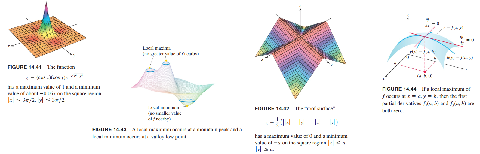
theorem 10—First Derivative Test for Local Extreme Values
If $ƒ(x, y)$ has a local maximum or minimum value at an interior point $(a, b)$ of its domain and if the first partial derivatives exist there, then $ƒ_x(a, b) = 0$ and $ƒ_y(a, b) = 0$.

Definition
An interior point of the domain of a function $ƒ(x, y)$ where both $ƒ_x$ and $ƒ_y$ are zero or where one or both of $ƒ_x$ and $ƒ_y$ do not exist is a critical point of $ƒ$.

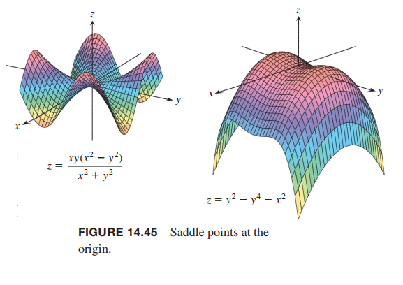
Definition
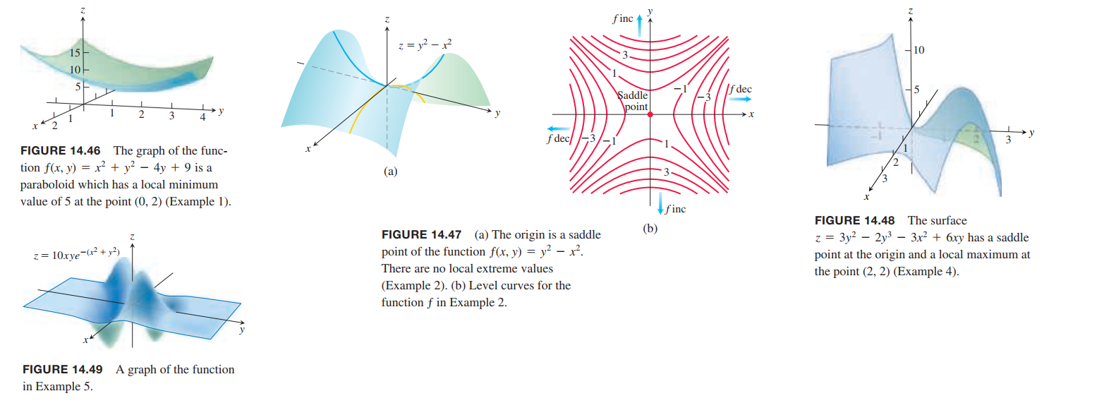
A differentiable function $ƒ(x, y)$ has a saddle point at a critical point $(a, b)$ if in every open disk centered at $(a, b)$ there are domain points $(x, y)$ where $ƒ(x, y) < ƒ(a, b)$ and domain points $(x, y)$ where $ƒ(x, y) > ƒ(a, b)$. The corresponding point $(a, b, ƒ(a, b))$ on the surface $z = ƒ(x, y)$ is called a saddle point of the surface (Figure 14.45).

theorem 11—Second Derivative Test for Local Extreme Values
Suppose that $ƒ(x, y)$ and its first and second partial derivatives are continuous throughout a disk centered at $(a, b)$ and that $f_x(a, b) = f_y(a, b) = 0$. Then
i) $f$ has a local maximum at $(a, b)$ if $f_{xx} < 0$ and $f_{xx} f_{yy} - f_{xy}^2 > 0$ at $(a, b)$.
ii) $f$ has a local minimum at $(a, b)$ if $f_{xx} > 0$ and $f_{xx} f_{yy} - f_{xy}^2 > 0$ at $(a, b)$.
iii) $f$ has a saddle point at $(a, b)$ if $f_{xx} f_{yy} - f_{xy}^2 < 0$ at $(a, b)$.
iv) the test is inconclusive at $(a, b)$ if $f_{xx} f_{yy} - f_{xy}^2 = 0$ at $(a, b)$. In this case, we must find some other way to determine the behavior of $f$ at $(a, b)$.

The expression $f_{xx} f_{yy} - f_{xy}^2$ is called the discriminant(判别式) or Hessian of $f$. It is sometimes easier to remember it in determinant form,
$$
f_{xx} f_{yy} - f_{xy}^2 =
\begin{vmatrix}
f_{xx} & f_{xy} \\
f_{xy} & f_{yy}
\end{vmatrix}
$$

Absolute Maxima and Minima on Closed Bounded Regions

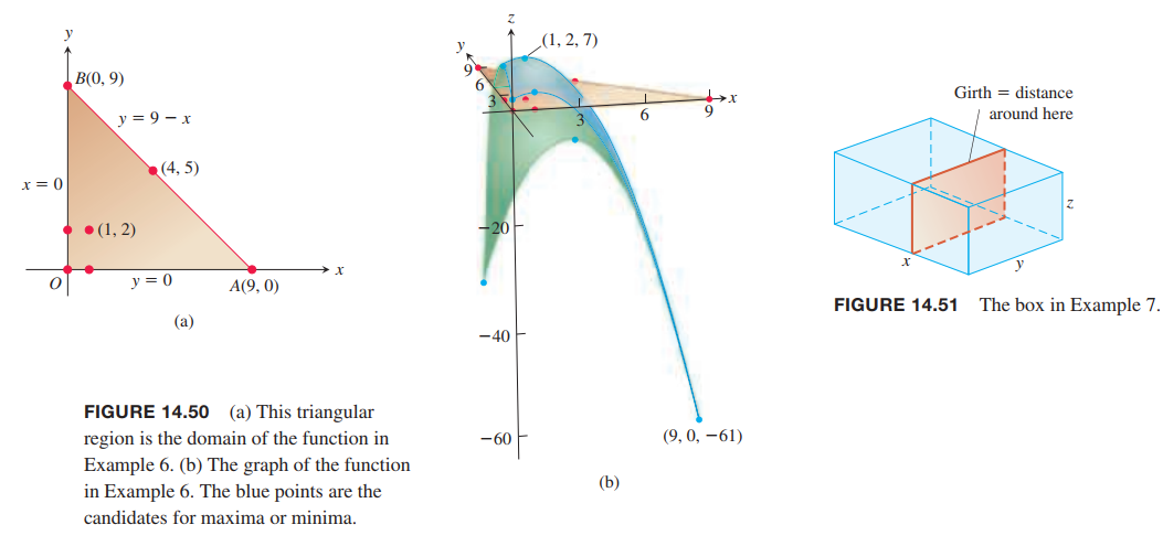
We organize the search for the absolute extrema of a continuous function $ƒ(x, y)$ on a closed and bounded region $R$ into three steps.

1. List the interior points of $R$ where $ƒ$ may have local maxima and minima and evaluate $ƒ$ at these points. These are the critical points of $ƒ$.
2. List the boundary points of $R$ where $ƒ$ has local maxima and minima and evaluate $ƒ$ at these points. We show how to do this in the next example.
3. Look through the lists for the maximum and minimum values of $ƒ$. These will be the absolute maximum and minimum values of $ƒ$ on $R$.

Lagrange Multipliers(拉格朗日乘子)

Here we explore a powerful method for finding extreme values of constrained functions: the method of Lagrange multipliers.

Constrained Maxima and Minima

💡For example💡:

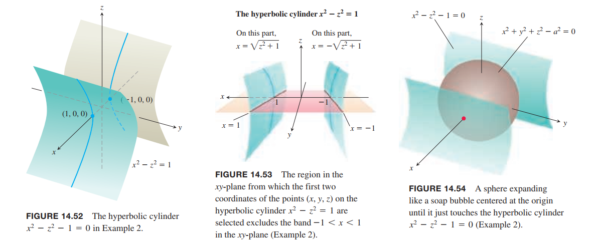
Find the points on the hyperbolic cylinder(双曲柱面) $x^2 - z^2 - 1 = 0$ that are closest to the origin.

Solution:

• Substitution.

This problems means, we are seeking the points whose coordinates minimize the value of the function $f(x,y,z) = x^2 + y^2 + z^2$ subject to the constraint that $x^2 - z^2 - 1 = 0$.

First, we try to regard $x$ and $y$ as independent variables, then $z^2 = x^2 - 1$.

So, the problem becomes we look for the points in the $xy$-plane whose coordinates minimize $h$.
$$
f(x,y,z) = x^2 + y^2 + z^2 \longmapsto \\
h(x,y) = x^2 + y^2 + (x^2-1) \\
= 2x^2 + y^2 -1
$$

By First Derivative Test
$$
h_x = 4x = 0, h_y = 2y = 0
$$
The point should be $(0,0)$.But there are no points on the cylinder where both $x$ and $y$ are zero. Why?

Although the domain of $h$ is the entire $xy$-plane, the domain from which we can select the first two coordinates of the points $(x, y, z)$ on the cylinder is restricted to the “shadow” of the cylinder on the $xy$-plane; it does not include the band between the lines $x = -1$ and $x = 1$ (Figure 14.53).

If we eliminate the one variable by

$$
x^2 = z^2 + 1\\
k(y,z) = 1 + y^2 + 2z^2
$$
we can get the right answer.

• Tangent plane and Normal line.

At each point of contact, the cylinder and sphere have the same tangent plane and normal line.

Therefore, if the sphere and cylinder are represented as the level surfaces obtained by setting

$$
f(x,y,z) = x^2 + y^2 + z^2 - a^2\\
g(x,y,z) = x^2 -z^2 - 1
$$
equal to 0.

Then the gradients $\nabla ƒ$ and $\nabla g$ will be parallel where the surfaces touch.
$$
\nabla f = \lambda \nabla g
$$
which is
$$
2x i + 2y j + 2z k = \lambda (2x i - 2zk)
$$
the solution point should satisfy
$$
\begin{cases}
2x = 2\lambda x\\
2y = 0\\
2z = -2\lambda z
\end{cases}
$$
and
$$
x^2 - z^2 - 1 = 0
$$
thus,
$$
\lambda = 1
$$

The points on the cylinder closest to the origin are the points $(\pm 1, 0, 0)$.

The Method of Lagrange Multipliers

THEOREM 12—The Orthogonal Gradient Theorem
Suppose that $ƒ(x, y, z)$ is differentiable in a region whose interior contains a smooth curve
$$
C: r(t) = x(t) i + y(t) j + z(t) k
$$
If $P_0$ is a point on $C$ where $ƒ$ has a local maximum or minimum relative to its values on $C$, then $\nabla f$ is orthogonal to $C$ at $P_0$.

COROLLARY
At the points on a smooth curve $r(t) = x(t)i + y(t)j$ where a differentiable function $ƒ(x, y)$ takes on its local maxima and minima relative to its values on the curve, $\nabla f \cdot r’ = 0$.

The Method of Lagrange Multipliers
Suppose that $ƒ(x, y, z)$ and $g(x, y, z)$ are differentiable and $\nabla g \neq 0$ when $g(x, y, z) = 0$. To find the local maximum and minimum values of $ƒ$ subject to the constraint $g(x, y, z) = 0$ (if these exist), find the values of $x, y, z$, and $l$ that simultaneously satisfy the equations
$$
\nabla f = \lambda \nabla g, and, g(x,y,z) = 0\tag{1}
$$
For functions of two independent variables, the condition is similar, but without the variable $z$.

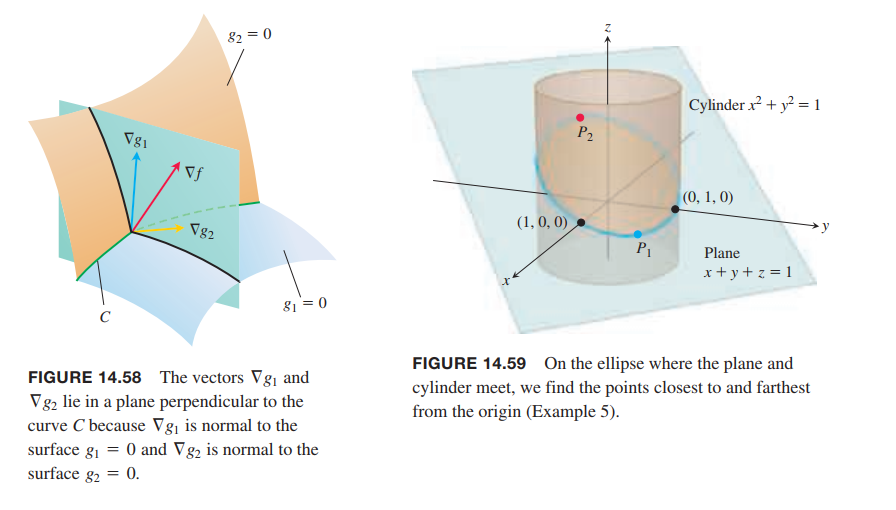
💡For example💡:

Find the greatest and smallest values that the function
$$
f(x,y) = xy
$$
takes on the ellipse (Figure 14.55)
$$
\frac{x^2}{8} + \frac{y^2}{2} = 1
$$

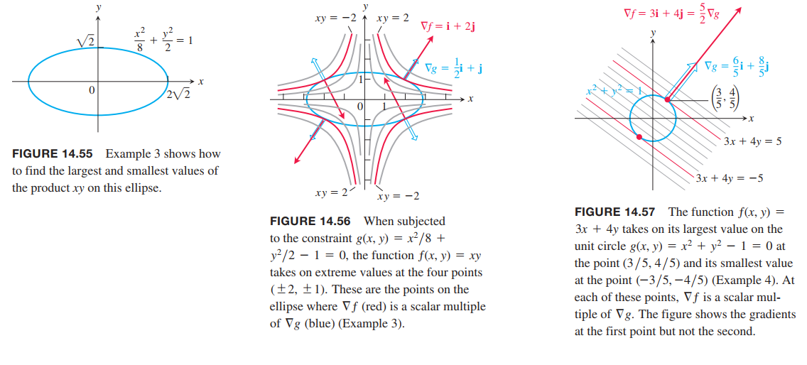
Solution:

the problem is abstracted as :

find the extreme values of $f(x,y) = xy$ subject to the constraint $g(x,y) = \frac{x^2}{8} + \frac{y^2}{2} - 1 = 0$.

$$
\nabla f = \lambda \nabla g, and, g(x,y) = 0
$$

$$
y i + x j = \lambda (\frac{1}{4}xi + yj)
$$

we find

$$
\begin{cases}
y = \frac{\lambda}{4}x\\
x = \lambda y
\end{cases}
$$
we get
$$
y = 0, or, \lambda = \pm 2
$$

Case1: $y = 0$. Then $x = 0, y = 0$. But this point is not on the ellipse. Hence, $y \neq 0$.

Case2:

$$
\lambda = \pm 2, x = \pm 2y
$$
$$
\frac{(\pm 2y)^2}{8} + \frac{y^2}{2} = 1, y = \pm 1
$$

So, The extreme values are $xy = 2$ and $xy = -2$.

Lagrange Multipliers with Two Constraints

$$
\nabla f = \lambda \nabla g_1 + \mu \nabla g_2, g_1(x,y,z)=0, g_2(x,y,z) = 0
\tag{2}
$$

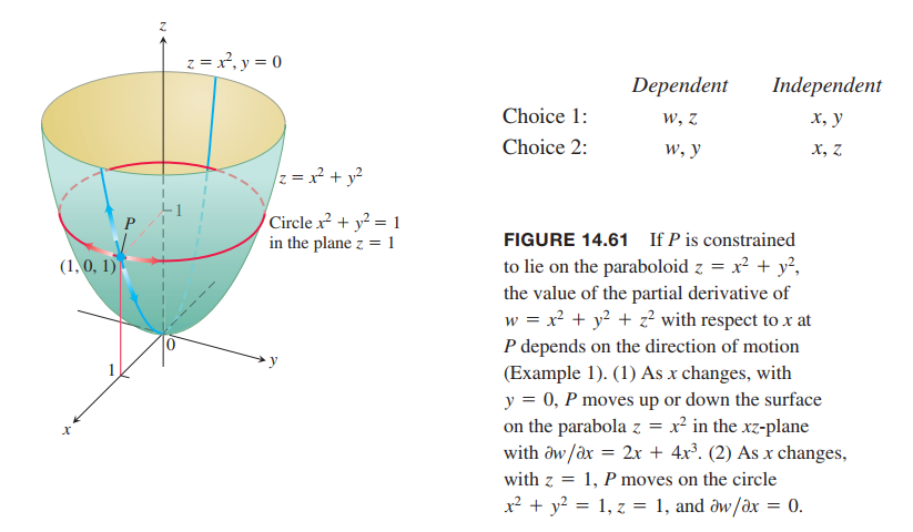
💡For example💡:
The plane $x + y + z = 1$ cuts the cylinder $x^2 + y^2 = 1$ in an ellipse (Figure 14.59). Find the points on the ellipse that lie closest to and farthest from the origin.

Solution:

The problem is abstracted as:

find the extreme values of $f(x,y,z) = x^2 + y^2 + z^2$ substract to the constraints

$$
g_1(x,y,z) = x^2 + y^2 - 1 = 0\\
g_2(x,y,z) = x + y + z = 0
$$

$$
\nabla f = \lambda \nabla g_1 + \mu \nabla g_2
$$
we get
$$
\begin{cases}
2x = 2\lambda x + \mu\\
2y = 2\lambda y + \mu\\
2z = \mu
\end{cases}
\longrightarrow
\begin{cases}
(1-\lambda)x = z\\
(1-\lambda)y = z
\end{cases}
\tag{6}
$$
the result is $\lambda = 1$ and $z = 0$, or $\lambda \neq 1$ and $x = y = \frac{z}{(1-\lambda)}$.

Case1. $z = 0$, we get $(1,0,0)$ and $(0,1,0)$.
Case2. $x = y$, we get $P_1(\frac{\sqrt 2}{2}, \frac{\sqrt 2}{2}, 1 - \sqrt{2})$ and $P_2(-\frac{\sqrt 2}{2}, -\frac{\sqrt 2}{2}, 1 + \sqrt{2})$

The points on the ellipse closest to the origin are $(1, 0, 0)$ and $(0, 1, 0)$. The point on the ellipse farthest from the origin is $P_2$. (See Figure 14.59.)

Taylor’s Formula for Two Variables

Derivation of the Second Derivative Test

The Error Formula for Linear Approximations

Taylor’s Formula for Functions of Two Variables

👉Taylor’s Formula for Single-Variable Function >>

Taylor’s Formula for $ƒ(x, y)$ at the Point $(a, b)$
Suppose $ƒ(x, y)$ and its partial derivatives through order $n + 1$ are continuous throughout an open rectangular region $R$ centered at a point $(a, b)$. Then, throughout $R$,
$$
\begin{aligned}
f(a+h,b+k) &= f(a,b) \\
&+ \left. (hf_x + kf_y)\right|_{(a,b)}\\
&+ \left. \frac{1}{2!}(h^2f_{xx} + 2hkf_{xy} + k^2f_{yy})\right|_{(a,b)} \\
&+ \left. \frac{1}{3!}(h^3f_{xxx} + 3h^2kf_{xxy} + 3hk^2f_{xyy} + k^3f_{yyy})\right|_{(a,b)} \\
&+ \cdots \\
&+ \left. \frac{1}{n!}(h\frac{\partial }{\partial x} + k \frac{\partial}{\partial y})^n f\right|_{(a,b)} \\
&+ \left. \frac{1}{(n+1)!}(h\frac{\partial}{\partial x} + k \frac{\partial}{\partial y})^{n+1} f\right|_{(a+ch,b+ck)}
\end{aligned}
\tag{7}
$$

Partial Derivatives with Constrained Variables

Decide Which Variables Are Dependent and Which Are Independent

💡For example💡:

Find $\partial w/\partial x$ if $w = x^2 + y^2 + z^2$ and $z = x^2 + y^2$.

Solution:

This is the formula for $\partial w / \partial x$ when $x$ and $y$ are the independent variables.
$$
\frac{\partial w}{\partial x} = 2x + 4x^3 + 4xy^2
$$
This is the formula for $\partial w / \partial x$ when $x$ and $z$ are the independent variables.
$$
\frac{\partial w}{\partial x} = 0
$$

How to Find $\partial w/ \partial x$ When the Variables in $w = ƒ(x, y, z)$ Are Constrained by Another Equation

1. Decide which variables are to be dependent and which are to be independent. (In practice, the decision is based on the physical or theoretical context of our work. In the exercises at the end of this section, we say which variables are which.)
2. Eliminate the other dependent variable(s) in the expression for $w$.
3. Differentiate as usual.

Notation

$\partial w / \partial x$ with $x$ and $y$ independent:
$$
(\frac{\partial w}{\partial x})_y
$$

$\partial w / \partial x$ with $x$ and $y$ and $t$ independent:
$$
(\frac{\partial w}{\partial x})_{y,t}
$$

Arrow Diagrams