Keywords: Euler’s Method, Slope Fields, Autonomous Equations
This is the Chapter9 ReadingNotes from book Thomas Calculus 14th.
Solutions, Slope Fields, and Euler’s Method
Many differential equations cannot be solved by obtaining an explicit formula for the solution. However, we can often find numerical approximations to solutions.
General First-Order Differential Equations and Solutions
A first-order differential equation is an equation
$$
\frac{dy}{dx} = f(x,y)
\tag{1}
$$
in which $ƒ(x, y)$ is a function of two variables defined on a region in the $xy$-plane. In a typical situation $y$ represents an unknown function of $x$, and $ƒ(x, y)$ is a known function. Such as:
$$
y’ = x + y, y’ = y / x, y’ = 3xy
$$
A solution of Equation (1) is a differentiable function y = y(x) defined on an interval $I$ of $x$-values (perhaps infinite) such that
$$
\frac{d}{dx}y(x) = f(x,y(x))
$$
💡For example💡:
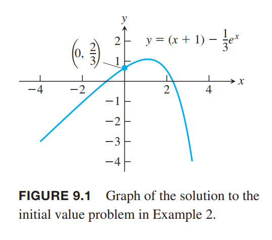
Show that the function $y = (x+1)-\frac{1}{3}e^x$ is a solution to the first-order initial value problem(一阶初值问题) $\frac{dy}{dx} = y-x, y(0) = \frac{2}{3}$
Solution:
The equation
$$
\frac{dy}{dx} = y-x
$$
is a first-order differential equation with $ƒ(x, y) = y - x$.
On the left side of the equation:
$$
\frac{dy}{dx} = \frac{d}{dx} (x+1-\frac{1}{3}e^x) = 1 - \frac{1}{3}e^x
$$
On the Right side of the equation:
$$
y-x = 1 - \frac{1}{3}e^x
$$
The function satisfies the initial condition because
$$
y(0) = [(x+1)-\frac{1}{3}e^x]_{x=0} = \frac{2}{3}
$$
The graph of the function is shown in Figure 9.1.
Slope Fields: Viewing Solution Curves
Each time we specify an initial condition $y(x_0) = y_0$ for the solution of a differential equation $y’ = ƒ(x, y)$, the solution curve (graph of the solution) is required to pass through the point $(x_0, y_0)$ and to have slope $ƒ(x_0, y_0)$ there. We can picture these slopes graphically by drawing short line segments of slope $ƒ(x, y)$ at selected points $(x, y)$ in the region of the $xy$ plane that constitutes the domain of $ƒ$. Each segment has the same slope as the solution curve through $(x, y)$ and so is tangent to the curve there. The resulting picture is called a slope field (or direction field) and gives a visualization of the general shape of the solution curves. Figure 9.2a shows a slope field, with a particular solution sketched into it in Figure 9.2b. We see how these line segments indicate the direction the solution curve takes at each point it passes through.
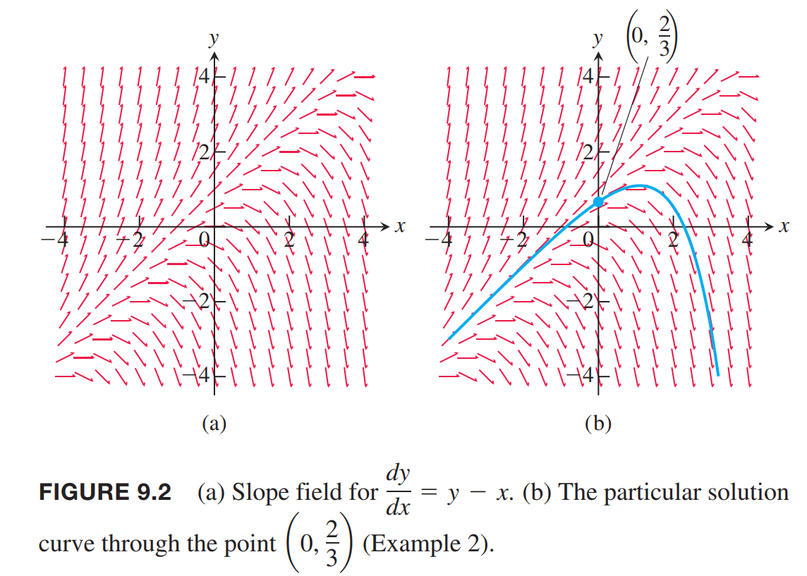
Slope fields are useful because they display the overall behavior of the family of solution curves for a given differential equation.
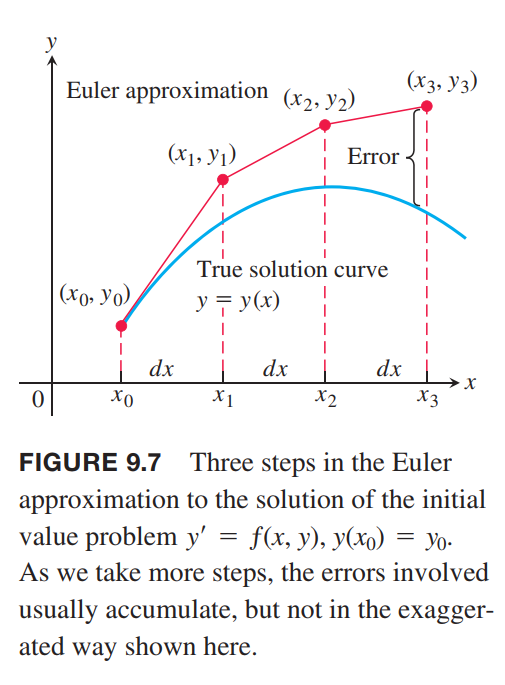
Euler’s Method
The basis of Euler’s method is to patch together a string of linearizations to approximate the curve over a longer stretch.(本质上还是数值分析, 迭代逼近)
Given a differential equation $dy/dx = ƒ(x, y)$ and an initial condition $y(x_0) = y_0$, we can approximate the solution $y = y(x)$ by its linearization
$$
L(x) = y(x_0) + y’(x_0)(x-x_0)
$$
or
$$
L(x) = y_0 + f(x_0, y_0)(x-x_0)
$$
💡For example💡:
Use Euler’s method to solve $y’ = 1 + y , y(0) = 1$, on the interval $0 \leq x \leq 1$, starting at $x_0 = 0$ and taking $dx = 0.1$, Compare the approximations with the values of the exact solution $y = 2e^x - 1$.
Solution:
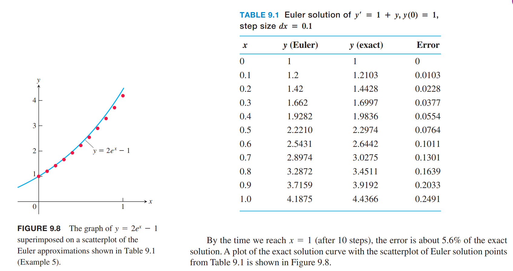
First:
$$
\begin{aligned}
y_1 &= y_0 + f(x_0,y_0)dx \\
&= y_0 + (1+y_0)dx\\
&= 1 + (1+1)(0.1)\\
&= 1.2
\end{aligned}
$$
Second:
$$
\begin{aligned}
y_2 &= y_1 + f(x_1,y_1)dx \\
&= y_1 + (1+y_1)dx\\
&= 1.2 + (1+1.2)(0.1)\\
&= 1.42
\end{aligned}
$$
First-Order Linear Equations
A first-order linear differential equation is one that can be written in the form
$$
\frac{dy}{dx} + P(x)y = Q(x)
$$
where $P$ and $Q$ are continuous functions of $x$. Equation (1) is the linear equation’s standard form
Solving Linear Equations
$v(x)$ is choosen to make $v\frac{dy}{dx} + Pvy = \frac{d}{dx}(v \cdot y)$:
$$
\begin{aligned}
&\frac{dy}{dx} + P(x)y = Q(x)\\
&v(x)\frac{dy}{dx} + P(x)v(x)y = v(x)Q(x)\\
&\frac{d}{dx}(v(x) \cdot y) = v(x)Q(x)\\
&v(x) \cdot y = \int v(x)Q(x)dx\\
&y = \frac{1}{v(x)} \int v(x)Q(x)dx
\end{aligned}
$$
about $v(x)$:
$$
\begin{aligned}
&\frac{d}{dx}(vy) = v\frac{dy}{dx} + yPv\\
&v\frac{dy}{dx} + y\frac{dv}{dx} = v\frac{dy}{dx} + yPv\\
&y\frac{dv}{dx} = yPv\\
&\frac{dv}{dx} = Pv\\
&\frac{dv}{v} = Pdx\\
&\int\frac{dv}{v} = \int Pdx\\
&\ln v = \int Pdx\\
&e^{\ln v} = e^{\int Pdx}\\
&v = e^{\int Pdx}
\end{aligned}
$$
Applications
Motion with Resistance Proportional to Velocity
Inaccuracy of the Exponential Population Growth Model
We model the population growth with the Law of Exponential Change:
$$
\frac{dP}{dt} = kP, P(0) = P_0
$$
where $P$ is the population at time $t$, $k > 0$ is a constant growth rate, and $P_0$ is the size of the population at time $t = 0$.
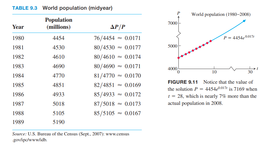
The solution is $P = P_0 e^{kt}$, the initial value is
$$
\frac{dP}{dt} = 0.017P, P(0) = 4454
$$
Orthogonal Trajectories
Graphical Solutions of Autonomous Equations(自控(自治)微分方程)
A differential equation for which $dy / dx$ is a function of $y$ only is called an autonomous differential equation.
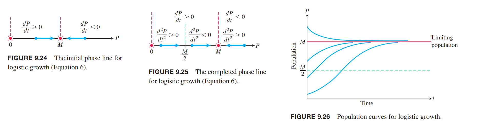
Logistic Population Growth
Without considering the carrying capacity of environment, the population growth can be modeled as
$$
\frac{dP}{dt} = kP, k-constant
\tag{5}
$$
Considering the environment factors, it should be
$$
k = r(M-P), r-constant
$$
where, $M$ is the maximum population it can carry.
thus,
$$
\frac{dP}{dt} = r(M-P)P = rMP-rP^2
\tag{6}
$$
The model given by Equation (6) is referred to as logistic growth(对数增长).
$$
\begin{aligned}
\frac{d^2P}{d^2t} &= \frac{d}{dt}(rMP-rP^2)\\
&= rM\frac{dP}{dt} - 2rP\frac{dP}{dt}\\
&= r(M-2P)\frac{dP}{dt}
\end{aligned}
$$
Systems of Equations and Phase Planes
To be added…

