Keywords: Interpolation, Quaternion, pipeline
This is the Chapter3 ReadingNotes from book Computer Animation_ Algorithms and Techniques_ Parent-Elsevier (2012).
Interpolation
The appropriate function
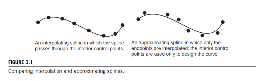
Interpolation versus approximation
Commonly used interpolating functions are the Hermite formulation and the Catmull-Rom spline.
Complexity
The simpler the underlying equations of the interpolating function, the faster its evaluation. In practice, polynomials are easy to compute, and piecewise cubic polynomials are the lowest degree polynomials that provide sufficient smoothness while still allowing enough flexibility to satisfy other constraints such as beginning and ending positions and tangents.
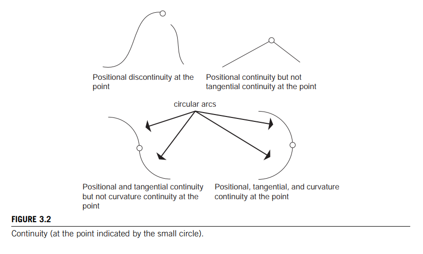
Continuity
Zero-order continuity refers to the continuity of values of the curve itself.
If the same can be said of the first derivative of the function (the instantaneous change in values of the curve), then the function has first-order, or tangential, continuity.
Second-order continuity refers to continuous curvature or instantaneous change of the tangent vector.
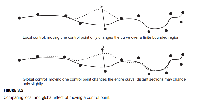
Global versus local control
A formulation in which control points have a limited effect on the curve is referred to as providing local control.
If repositioning one control point redefines the entire curve, however slightly, then the formulation provides only global control.
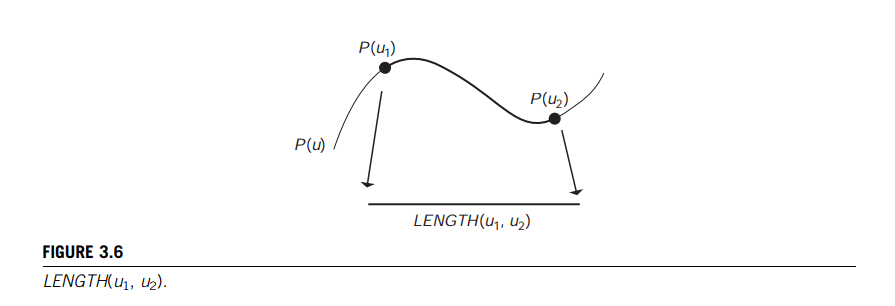
Controlling the motion of a point along a curve
for a given value of $u$, will produce a value that is a point in space, that is, $\pmb{p} = \pmb{P(u)}$.
for any specified time, $u$, a position $(X, Y, Z)$ can be produced as $(P_x(u), P_y(u), P_z(u)) = P(u)$.
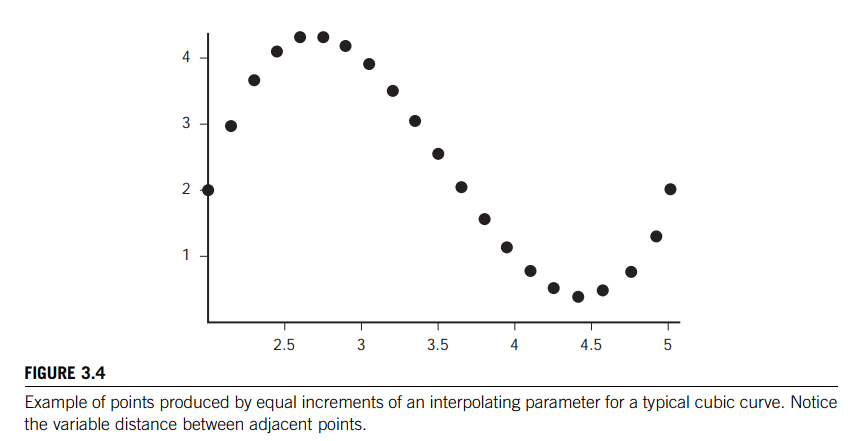
If positions are being interpolated by varying $u$ at a constant rate, the positions that are generated will not necessarily, in fact will seldom, represent a constant speed (e.g., see Figure 3.4).
To ensure a constant speed for the interpolated value, the interpolating function has to be parameterized by arc length, that is, distance along the curve of interpolation.
Computing arc length
Alternatively, instead of specifying time constraints, the animator might want to specify the relative velocities that an object should have along the curve.
It is important to remember that in animation the path swept out by the curve in space is not the only important thing. Equally important is how the path is swept out over time.
The analytic approach to computing arc length
The length of the curve from a point $\pmb{P}(u_a)$ to any other point $\pmb{P}(u_b)$ can be found by evaluating the arc length integral [4] by
$$
s = \int_{u_a}^{u_b} |dP/du| du
\tag{3.3}
$$
where the derivative of the space curve with respect to the parameterizing variable is defined to be
that shown in Equations 3.4 and 3.5.
$$
d\pmb{P} / du = ((dx(u)/(du)), (dy(u)/(du)), (dz(u)/(du)))
\tag{3.4}
$$
$$
|d\pmb{P} / du| = \sqrt{(dx(u)/du)^2 + (dy(u)/du)^2 + (dz(u)/du)^2}
\tag{3.5}
$$
👉Space Arc Length in Calculus >>
Estimating arc length by forward differencing
As mentioned previously, analytic techniques are not tractable for many curves of interest to animation.
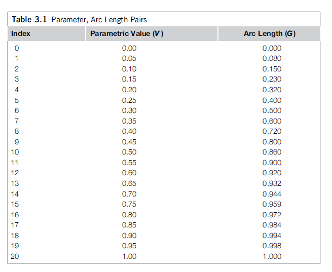
The easiest and conceptually simplest strategy for establishing the correspondence between parameter value and arc length is to sample the curve at a multitude of parametric values.
💡 for example💡:
the user wants to know the distance (arc length) from the beginning of the curve to the point on the curve corresponding to a parametric value of 0.73.
Solution:
The parametric entry closest to 0.73 must be located in the table. Since the parametric entries are evenly spaced, the distance between parametric entries is
$$
d = 0.05
$$
thus, the idex $i$,
$$
\begin{aligned}
i &= \lfloor \frac{v}{d} + 0.5 \rfloor \\&= \lfloor \frac{0.73}{0.05} + 0.5 \rfloor \\ &= 15
\end{aligned}
$$
A better approximation can be obtained by interpolating between the arc lengths corresponding to entries on either side of the given parametric value.
$$
i = \lfloor \frac{v}{d} \rfloor = 14
$$
thus,
$$
\begin{aligned}
s &= G[i] + \frac{v - V[i]}{V[i+1]-V[i]}(G[i+1]-G[i])\\
&= 0.944 + \frac{0.73-0.70}{0.75-0.70}(0.959-0.944)\\
&= 0.953
\end{aligned}
$$
What if given the arc length, I want to know the corresponding parameter value?
💡 for example💡:
Estimate the location of the point on the curve that is 0.75 unit of arc length from the beginning of the curve.
Solution:
the value of 0.75 is three-eighths of the way between the table values 0.72 and 0.80. An estimate of the parametric value would be calculated as
$$
u = 0.40 + \frac{3}{8}(0.45 - 0.40) = 0.41875
$$
Advantage: easy to implement, intuitive, fast to compute.
Disadvantage: errors.
- The curve can be supersampled to help reduce errors in forming the table.
- Instead of linear interpolation, higher-degree interpolation procedures can be used in computing the parametric value.
Adaptive approach
The adaptive approach begins by initializing the table with an entry for the first point of the curve, $<0.0, P(0)>$, and initializing the list of segments to be tested with the entire curve, $<0.0,1.0>$.
The segment’s midpoint is computed by evaluating the curve at the middle of the range of its parametric value. The curve is also evaluated at the endpoint of the segment; the position of the start of the segment is already in the table and can be retrieved from there.
$$
|||P(0.0) - P(1.0)|| - (||P(0.0) - P(0.5)|| + ||P(0.5) - P(1.0)||)| < \epsilon
$$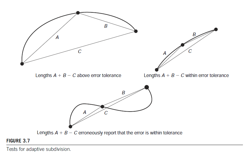
If the difference between these two values is above some user-specified threshold, then both halves, in order, are added to the list of segments to be tested along with their error tolerance ($\epsilon/2^n$ where $n$ is the level of subdivision).
If the values are within tolerance, then the parametric value of the midpoint is recorded in the table along with the arc length of the first point of the segment plus the distance from the first point to the midpoint.
Also added to the table is the last parametric value of the segment along with the arc length to the midpoint plus the distance from the midpoint to the last point.
When the list of segments to be tested becomes empty, a list of $<$parametric value, arc length$>$ has been generated for the entire curve.
Estimating the arc length integral numerically
Many numerical integration techniques approximate the integral of a function with the weighted sum of values of the function at various points in the interval of integration.
Techniques such as Simpson’s and trapezoidal integration use evenly spaced sample intervals. Gaussian quadrature [1] uses unevenly spaced intervals in an attempt to get the greatest accuracy using the smallest number of function evaluations.
👉Numerical Differentiation and Integration >>
$$
\begin{aligned}
&\int_{-1}^{1} f(u) = \sum_i w_i f(u_i)\\
&t = f(u) = \frac{(b-a)}{2}u + \frac{b+a}{2}\\
&\int_a^b g(t) dt = \int_{-1}^{1}g(\frac{(b-a)}{2}u + \frac{b+a}{2})du
\end{aligned}
$$
Adaptive Gaussian integration
Adaptive Gaussian integration is similar to the previously discussed adaptive forward differencing.
Find a point that is a given distance along a curve
Speed control
Ease-in/ease-out
Sine interpolation
Using sinusoidal pieces for acceleration and deceleration
Single cubic polynomial ease-in/ease-out
Constant acceleration: parabolic ease-in/ease-out

