Keywords: Bayesian Networks, Markov Random Fields, Inference, Python
This is the Chapter8 ReadingNotes from book Bishop-Pattern-Recognition-and-Machine-Learning-2006. [Code_Python]
We shall find it highly advantageous to augment the analysis using diagrammatic representations of probability distributions, called probabilistic graphical models. These offer several useful properties:
- They provide a simple way to visualize the structure of a probabilistic model and can be used to design and motivate new models.(直观的看到概率模型的结构,可以推动设计新的模型)
- Insights into the properties of the model, including conditional independence properties, can be obtained by inspection of the graph.(直观的看到概率模型的属性,包括条件独立等)
- Complex computations, required to perform inference and learning in sophisticated models, can be expressed in terms of graphical manipulations, in which underlying mathematical expressions are carried along implicitly.(通过图计算,可以表达复杂的数学计算,推断学习等过程)
Bayesian Networks
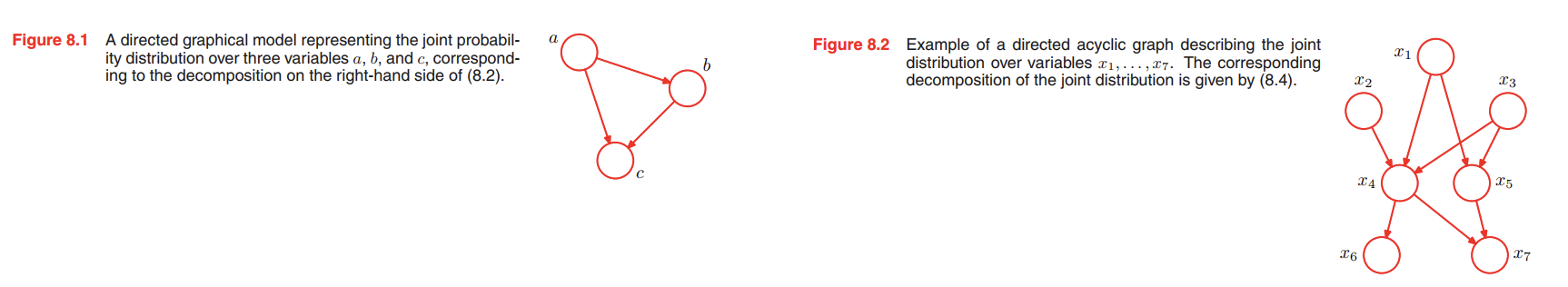
Consider first an arbitrary joint distribution $p(a, b, c)$ over three variables $a, b$, and $c$. By application of the product rule of probability (1.11), we can write the joint distribution in the form
$$
\begin{aligned}
p(a,b,c) &= p(c|a,b)p(a,b)\\
&= p(c|a,b)p(b|a)p(a)
\end{aligned}
\tag{8.2}
$$
By repeated application of the product rule of probability, this joint distribution can be written as a product of conditional distributions, one for each of the variables
$$
p(x_1, \cdots, x_K) = p(x_k|x_1,\cdots, x_{K-1})\cdots p(x_2|x_1)p(x_1)
\tag{8.3}
$$
We say that this graph is fully connected because there is a link between every pair of nodes.
See Figure8.2, the joint distribution of all 7 variables is therefore given by
$$
p(x_1)p(x_2)p(x_3)p(x_4|x_1, x_2, x_3)p(x_5|x_1, x_3)p(x_6|x_4)p(x_7|x_4, x_5)
\tag{8.4}
$$
Thus, for a graph with $K$ nodes, the joint distribution is given by
$$
p(\pmb{x}) = \prod_{k=1}^{K} p(x_k | pa_k)
\tag{8.5}
$$
where $pa_k$ denotes the set of parents of $x_k$, and $\pmb{x} = \lbrace x_1, \cdots , x_K \rbrace$. This key equation expresses the factorization properties of the joint distribution for a directed graphical model.
Example: Polynomial regression
We consider the 👉Bayesian polynomial regression model >>.
Random Variables in this model: the vector of polynomial coefficients $\pmb{w}$, the observed data $T = (t_1, \cdots , t_N)^T$.
Parameters in this model: the input data $X = (x_1, \cdots , x_N)^T$, the noise variance $\sigma^2$, the hyperparameter $\alpha$ representing the precision of the Gaussian prior over $\pmb{w}$.
Note that, the parameters definition here is a little different from before. We usually say $\pmb{w}$ is a parameter and $T$ is the observation/target data in Chaper 1.
we see that the joint distribution is given by the product of the prior $p(\pmb{w})$ and $N$ conditional distributions $p(t_n|\pmb{w})$ for $n = 1, \cdots , N$ so that
$$
p(T,\pmb{w}) = p(\pmb{w})\prod_{n=1}^N p(t_n|\pmb{w})
\Longleftrightarrow
p(T,\pmb{w}|X,\alpha,\sigma^2) = p(\pmb{w}|\alpha) \prod_{n=1}^N p(t_n|\pmb{w}, x_n, \sigma^2)
\tag{8.6}
$$
Correspondingly, we can make $X$ and $\alpha$ explicit in the graphical representation.
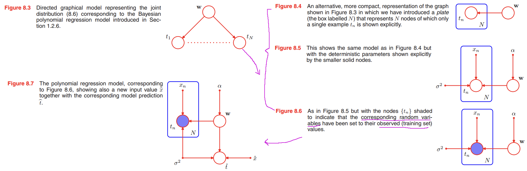
Note that the value of $\pmb{w}$ is not observed, and so $\pmb{w}$ is an example of a latent variable, also known as a hidden variable.
Having observed the values $\lbrace t_n \rbrace$ we can, if desired, evaluate the posterior distribution of the polynomial coefficients $\pmb{w}$ as discussed before. For the moment, we note that this involves a straightforward application of 👉Bayes’ theorem >>
$$
p(\pmb{w}|T) \propto p(\pmb{w})\prod_{n=1}^N p(t_n|\pmb{w})
\tag{8.7}
$$
Suppose we are given a new input value $\hat{x}$ and we wish to find the corresponding probability distribution for $\hat{t}$ conditioned on the observed data.
the corresponding joint distribution of all of the random variables in this model, conditioned on the deterministic parameters, is then given by
$$
p(\hat{t}, T, \pmb{w} | \hat{x}, X, \alpha, \sigma^2) = \left[ \prod_{n=1}^{N}p(t_n|x_n, \pmb{w}, \sigma^2) \right] p(\pmb{w}|\alpha) p(\hat{t}|\hat{x}, \pmb{w}, \sigma^2)
\tag{8.8}
$$
The required predictive distribution for $\hat{t}$ is then obtained, from the sum rule of probability, by integrating out the model parameters $\pmb{w}$ so that
$$
p(\hat{t}|\hat{x}, X,T, \alpha, \sigma^2) \propto \int p(\hat{t}, T, \pmb{w} | \hat{x}, X, \alpha, \sigma^2) d\pmb{w}
$$
where we are implicitly setting the random variables in $T$ to the specific values observed in the data set.
Generative models
Consider a joint distribution $p(x_1, \cdots, x_K)$ over $K$ variables that factorizes according to (8.5) corresponding to a directed acyclic graph. Our goal is to draw a sample $\hat{x_1}, \cdots, \hat{x_k}$ from the joint distribution.
- we start with the lowest-numbered node and draw a sample from the distribution $p(x_1)$, which we call $\hat{x_1}$.
- then work through each of the nodes in order, so that for node $n$ we draw a sample from the conditional distribution $p(x_n|pa_n)$ in which the parent variables have been set to their sampled values.
- Once we have sampled from the final variable $x_K$, we will have achieved our objective of obtaining a sample from the joint distribution.
We can interpret such models as expressing the processes by which the observed data arose. For instance, consider an object recognition task in which each observed data point corresponds to an image (comprising a vector of pixel intensities) of one of the objects. In this case, the latent variables might have an interpretation as the position and orientation of the object.
Given a particular observed image, our goal is to find the posterior distribution over objects, in which we integrate over all possible positions and orientations. We can represent this problem using a graphical model of the form show in Figure 8.8.
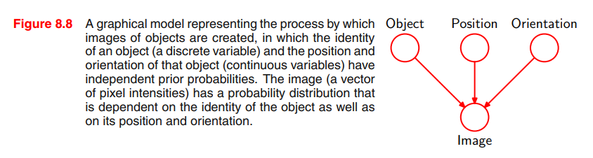
The graphical model captures the causal process (Pearl, 1988) by which the observed data was generated. For this reason, such models are often called generative models.
By contrast, the polynomial regression model described by Figure 8.5 is not generative because there is no probability distribution associated with the input variable $x$, and so it is not possible to generate synthetic data points from this model. We could make it generative by introducing a suitable prior distribution $p(x)$, at the expense of a more complex model.
Discrete variables
👉First to know Exponential Family >>
The probability distribution $p(x|\mu)$ for a single discrete variable $x$ having $K$ possible states (using the 1-of-K representation) is given by
$$
p(x|\mu) = \prod_{k=1}^K \mu_k^{x_k}
\tag{8.9}
$$
and is governed by the parameters $\mu = (\mu_1, \cdots , \mu_K)^T$.

