Keywords: K-means Clustering, Mixtures of Gaussians, EM Algorithm, Python
This is the Chapter9 ReadingNotes from book Bishop-Pattern-Recognition-and-Machine-Learning-2006. [Code_Python]
K-means Clustering
For each data point $\pmb{x_n}$, we introduce a corresponding set of binary indicator variables $r_{nk} \in \left\{ 0, 1 \right\}$, where $k = 1, \cdots , K$ describing which of the $K$ clusters the data point $\pmb{x_n}$ is assigned to, so that if data point $\pmb{x_n}$ is assigned to cluster $k$ then $r_{nk} = 1$, and $r_{nj} = 0$ for $j \neq k$. This is known as the $1-of-K$ coding scheme. We can then define an objective function, sometimes called a distortion measure, given by
$$
J = \sum_{n=1}^N \sum_{k=1}^K r_{nk} ||\pmb{x_n} - \pmb{\mu_k}||^2
\tag{9.1}
$$
which represents the sum of the squares of the distances of each data point to its assigned vector $\pmb{\mu_k}$.Our goal is to find values for the $\left\{ r_{nk} \right\}$ and the $\left\{ \pmb{\mu_{nk}} \right\}$ so as to minimize $J$.
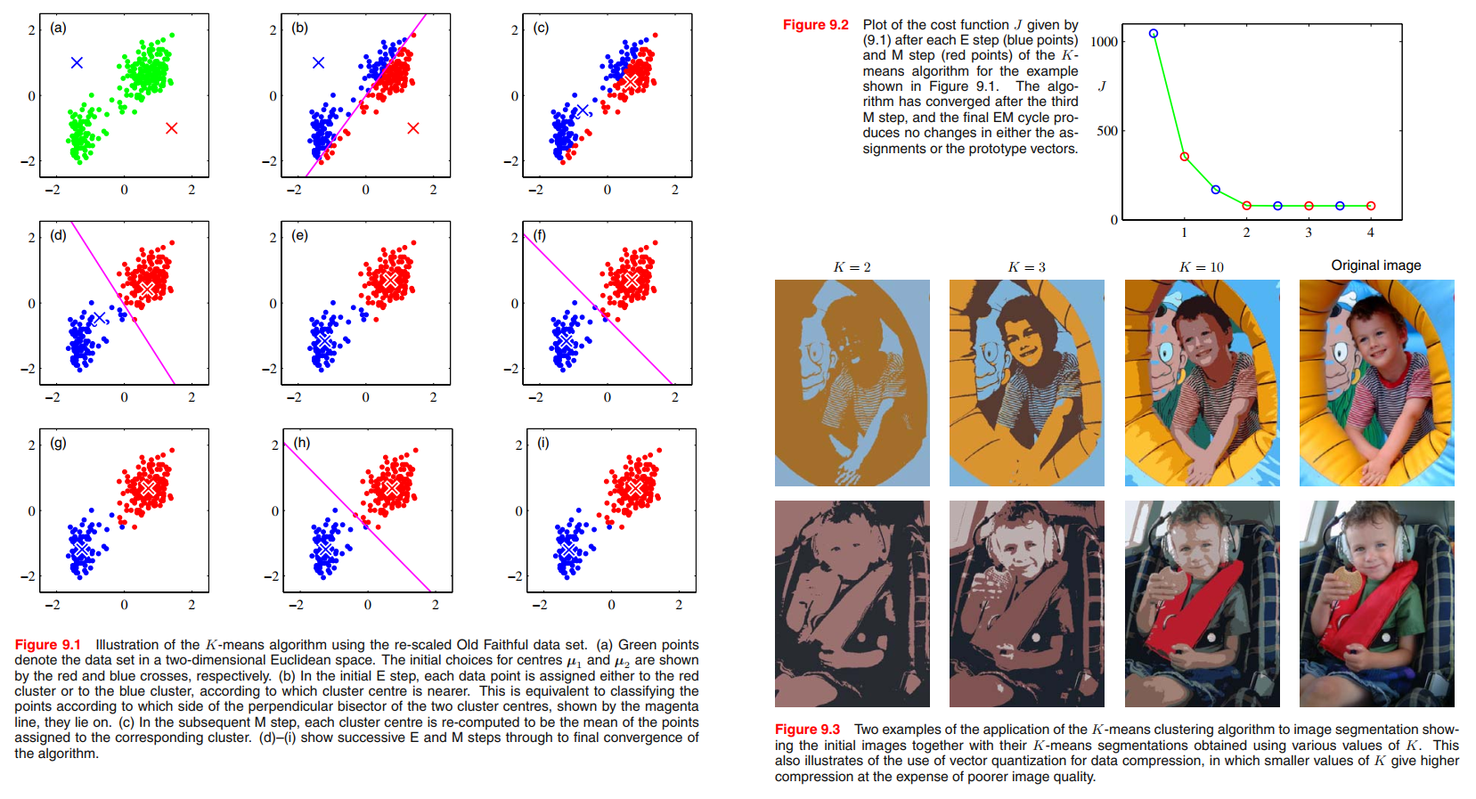
Image segmentation and compression
Mixtures of Gaussians
👉First Understanding Mixtures of Gaussians >>
We now turn to a formulation of Gaussian mixtures in terms of discrete latent variables.
Gaussian mixture distribution can be written as a linear superposition of Gaussians in the form,
$$
p(\pmb{x}) = \sum_{k=1}^K \pi_k \mathcal{N}(\pmb{x|\mu_k}, \pmb{\Sigma_k})
\tag{9.7}
$$
Proof:
Let us introduce a $K$-dimensional binary random variable $\pmb{z}$ having a $1$-of-$K$ representation in which a particular element $z_k$ is equal to $1$ and all other elements are equal to $0$.
The marginal distribution over $\pmb{z}$ is specified in terms of the mixing coefficients $\pi_k$, such that
$$
p(z_k = 1) = \pi_k
$$
where the parameters $\left\{ \pi_k \right\}$ must satisfy
$$
0 \leq \pi_k \leq 1
\tag{9.8}
$$
together with
$$
\sum_{k=1}^K \pi_k = 1
\tag{9.9}
$$
in order to be valid probabilities.
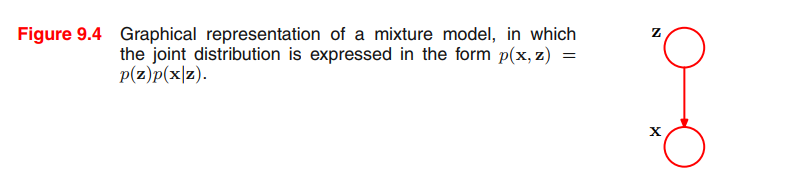
We shall define the joint distribution $p(\pmb{x}, \pmb{z})$ in terms of a marginal distribution $p(\pmb{z})$ and a conditional distribution $p(\pmb{x}|\pmb{z})$, corresponding to the graphical model in Figure 9.4.
👉More About $\pmb{\Sigma}$ Meaning >>
Because $\pmb{z}$ uses a $1$-of-$K$ representation, we can also write this distribution in the form
$$
p(\pmb{z}) = \prod_{k=1}^K \pi_k^{z_k}
\tag{9.10}
$$
Similarly, the conditional distribution of $\pmb{x}$ given a particular value for $\pmb{z}$ is a Gaussian
$$
p(\pmb{x}|z_k = 1) = \mathcal{N}(\pmb{x}|\pmb{\mu_k}, \pmb{\Sigma_k})
$$
$$
p(\pmb{x}|\pmb{z}) = \prod_{k=1}^K \mathcal{N}(\pmb{x}| \pmb{\mu_k}, \pmb{\Sigma_k})^{z_k}
\tag{9.11}
$$
the marginal distribution of $\pmb{x}$ is then obtained by summing the joint distribution over all possible states of $\pmb{z}$ to give
$$
\begin{aligned}
p(\pmb{x}) &= \sum_{\pmb{z}} p(\pmb{z}) p(\pmb{x}|\pmb{z}) \\
&= \sum_{k=1}^K \pi_k \mathcal{N}(\pmb{x} | \pmb{\mu_k}, \pmb{\Sigma_k})
\end{aligned}
\tag{9.12}
$$
Thus the marginal distribution of $\pmb{x}$ is a Gaussian mixture of the form (9.7).
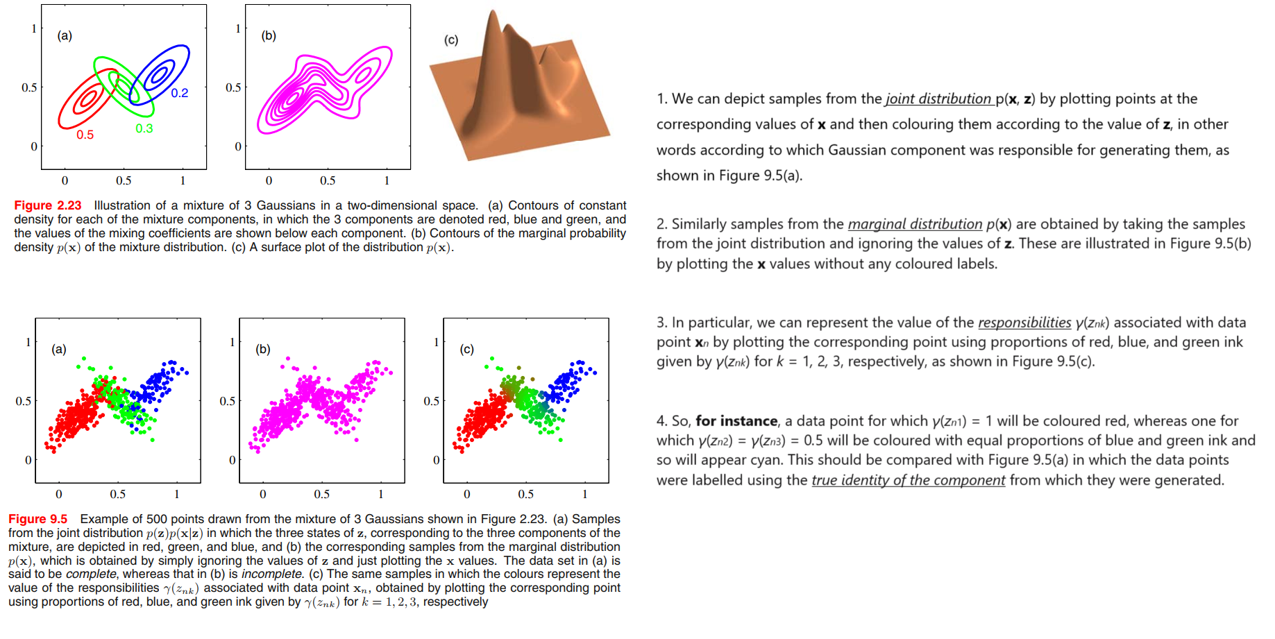
because we have represented the marginal distribution in the form $p(\pmb{x}) = \sum_{\pmb{z}} p(\pmb{x}, \pmb{z})$, it follows that for every observed data point $\pmb{x_n}$ there is a corresponding latent variable $\pmb{z_n}$.
We shall use $\gamma(z_k)$ to denote $p(z_k = 1| \pmb{x})$, whose value can be found using Bayes’ theorem
$$
\begin{aligned}
\gamma(z_k) & \equiv p(z_k = 1 | \pmb{x})\\
&= \frac{p(z_k = 1) p(\pmb{x}|z_k=1)}{\sum_{j=1}^K p(z_j = 1)p(\pmb{x} | z_j = 1)} \\
&= \frac{\pi_k \mathcal{N}(\pmb{x} | \pmb{\mu_k}, \pmb{\Sigma_k})}{\sum_{j=1}^K \pi_j \mathcal{N}(\pmb{x} | \pmb{\mu_j}, \pmb{\Sigma_j})}
\end{aligned}
\tag{9.13}
$$
prior probability of $z_k = 1$: $\pi_k$
posterior probability: $\gamma(z_k)$ once we have observed $\pmb{x}$.
$\gamma(z_k)$ can also be viewed as the responsibility that component $k$ takes for ‘explaining’ the observation $\pmb{x}$.
Maximum likelihood
$\pmb{X}$: $N \times D$ matrix, in which the $n^{th}$ row is given by $\pmb{x_n}^T$.
$\pmb{Z}$: $N \times K$ matrix, in which the $n^{th}$ row is given by $\pmb{z_n}^T$.
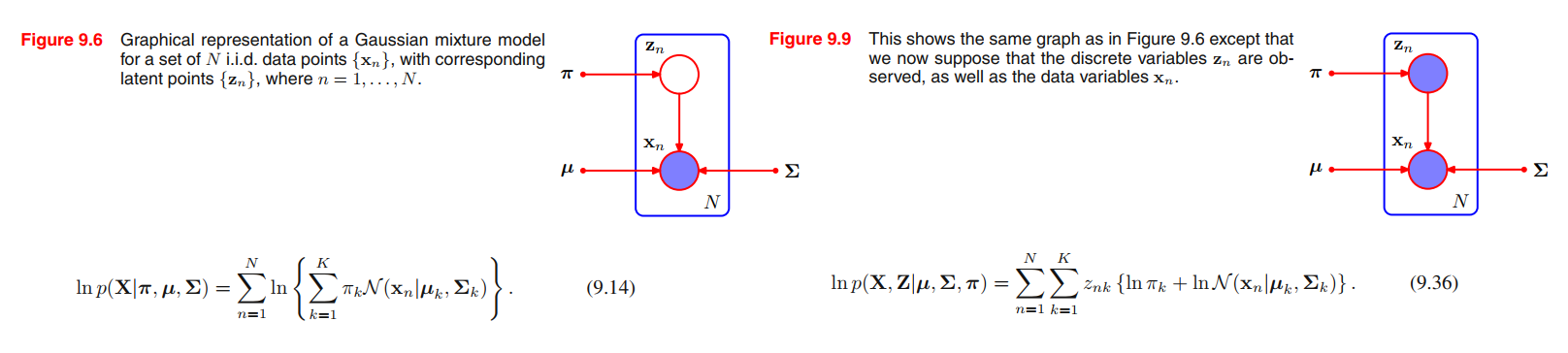
If we assume that the data points are drawn independently from the distribution, then we can express the Gaussian mixture model for this i.i.d. data set using the graphical representation shown in Figure 9.6. From (9.7) the log of the likelihood function is given by
$$
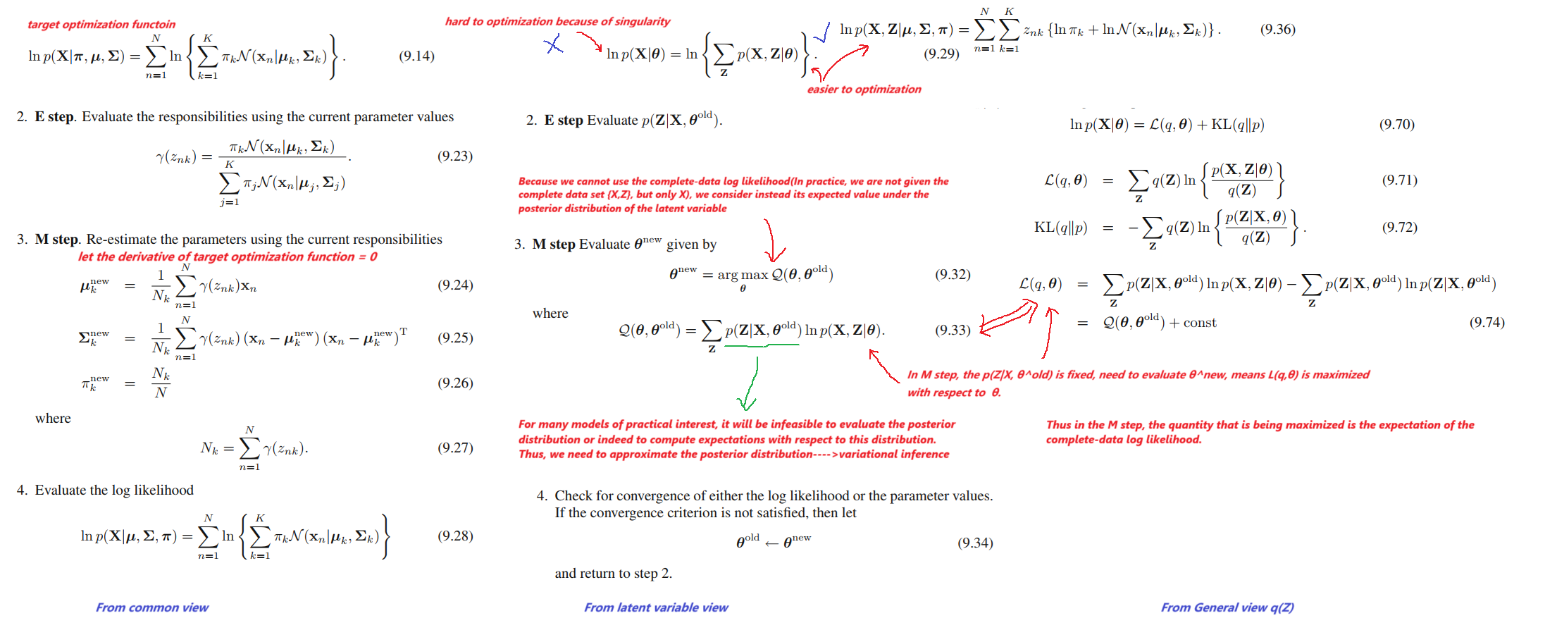
\ln p(\pmb{X} | \pmb{\pi}, \pmb{\mu}, \pmb{\Sigma}) = \sum_{n=1}^{N} \ln \left\{ \sum_{k=1}^{K} \pi_k \mathcal{N}(\pmb{x_n} | \pmb{\mu_k}, \pmb{\Sigma_k}) \right\}
\tag{9.14}
$$
Consider a Gaussian mixture whose components have covariance matrices given by $\pmb{\Sigma_k} = \sigma_k^2 \pmb{I}$, where $\pmb{I}$ is the unit matrix.
Suppose that one of the components of the mixture model, let us say the $j^{th}$ component, has its mean $\pmb{\mu_j}$ exactly equal to one of the data points so that $\pmb{\mu_j} = \pmb{x_n}$ for some value of $n$.
This data point will then contribute a term in the likelihood function of the form
$$
\mathcal{N}(\pmb{x_n} | \pmb{x_n}, \sigma_j^2 \pmb{I}) = \frac{1}{(2\pi)^{\frac{1}{2}}} \frac{1}{\sigma_j}
\tag{9.15}
$$
If we consider the limit $\sigma_j \rightarrow 0$, then we see that this term goes to infinity and so the log likelihood function will also go to infinity.
Thus the maximization of the log likelihood function is not a well posed problem because such singularities will always be present and will occur whenever one of the Gaussian components ‘collapses’ onto a specific data point.
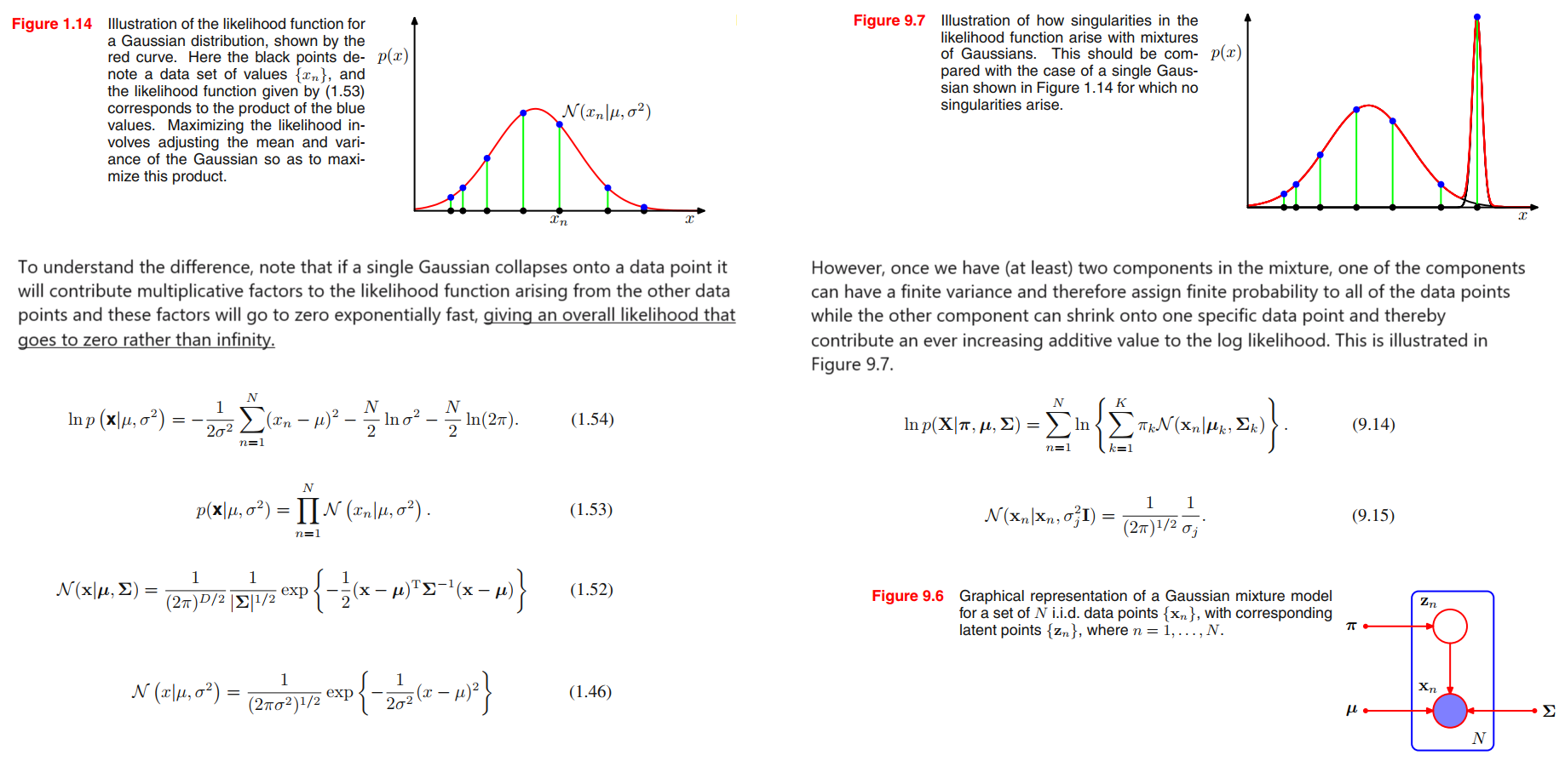
如果单个高斯函数折叠到一个数据点上,它将对由其他数据点产生的似然函数产生乘性因子,这些因子将以指数形式快速趋于零,从而使总体似然函数趋于零而不是无穷。
然而,一旦我们在混合中有(至少)两个成分,其中一个成分可能具有有限的方差,因此为所有数据点分配有限的概率,而另一个成分可以缩小到一个特定的数据点,从而为对数似然提供越来越大的附加值。
EM for Gaussian mixtures(without latent view)
An elegant and powerful method for finding maximum likelihood solutions for
models with latent variables is called the expectation-maximization algorithm, or EM
algorithm (Dempster et al., 1977; McLachlan and Krishnan, 1997).
Setting the derivatives of $\ln p(\pmb{X}|\pmb{\pi}, \pmb{\mu}, \pmb{\Sigma})$ in (9.14) with respect to the means $\pmb{\mu_k}$ of the Gaussian components to zero, we obtain
$$
0 = -\sum_{n=1}^N \underbrace{\frac{\pi_k \mathcal{N}(\pmb{x_n} | \pmb{\mu_k}, \pmb{\Sigma_k})}{\sum_j \pi_j \mathcal{N}(\pmb{x_n} | \pmb{\mu_j}, \pmb{\Sigma_j})}}_{\gamma(z_{nk})} \pmb{\Sigma_k}(\pmb{x_n} - \pmb{\mu_k})
\tag{9.16}
$$
Multiplying by $\pmb{\Sigma_k^{-1}}$ (which we assume to be nonsingular) and rearranging we obtain
$$
\pmb{\mu_k} = \frac{1}{N_k} \sum_{n=1}^{N} \gamma(z_{nk})\pmb{x_n}
\tag{9.17}
$$
where,
$$
N_k = \sum_{n=1}^{N} \gamma(z_{nk})
\tag{9.18}
$$
$N_k$ : effective number of points assigned to cluster $k$.
$\pmb{\mu_k}$: take a weighted mean of all of the points in the data set, in which the weighting factor for data point $\pmb{x_n}$ is given by the posterior probability $\gamma(z_{nk})$ that component $k$ was responsible for generating $\pmb{x_n}$.
Similar, we maximize $\ln p(\pmb{X}|\pmb{\pi}, \pmb{\mu}, \pmb{\Sigma})$ with respect to the mixing coefficients $\pmb{\Sigma_k}$,
$$
\pmb{\Sigma_k} = \frac{1}{N_k} \sum_{n=1}^N \gamma(z_{nk}) (\pmb{x_n} - \pmb{\mu_k})(\pmb{x_n} - \pmb{\mu_k})^T
\tag{9.19}
$$
Similar, we maximize $\ln p(\pmb{X}|\pmb{\pi}, \pmb{\mu}, \pmb{\Sigma})$ with respect to the mixing coefficients $\pi_k$, Here we must take account of the constraint (9.9), which requires the mixing coefficients to sum to one.
$$
\begin{cases}
\ln p(\pmb{X} | \pmb{\pi}, \pmb{\mu}, \pmb{\Sigma}) = \sum_{n=1}^{N} \ln \left\{ \sum_{k=1}^{K} \pi_k \mathcal{N}(\pmb{x_n} | \pmb{\mu_k}, \pmb{\Sigma_k}) \right\} \\
\sum_{k=1}^K \pi_k = 1
\end{cases}
$$
This can be achieved using a 👉Lagrange multiplier >> and maximizing the following quantity
$$
\ln p(\pmb{X} | \pmb{\pi}, \pmb{\mu}, \pmb{\Sigma}) + \lambda (\sum_{k=1}^K \pi_k - 1)
$$
which gives
$$
0 = \sum_{n=1}^{N} \frac{\mathcal{N}(\pmb{x_n} | \pmb{\mu_k}, \pmb{\Sigma_k})}{\sum_j \pi_j \mathcal{N}(\pmb{x_n} | \pmb{\mu_j}, \pmb{\Sigma_j})} + \lambda
\tag{9.21}
$$
we get
$$
\pi_k = \frac{N_k}{N}
\tag{9.22}
$$
so that the mixing coefficient for the $k$th component is given by the average responsibility which that component takes for explaining the data points.
It is worth emphasizing that the results (9.17), (9.19), and (9.22) do not constitute a closed-form solution for the parameters of the mixture model because the responsibilities $\gamma(z_{nk})$ depend on those parameters in a complex way through (9.13).
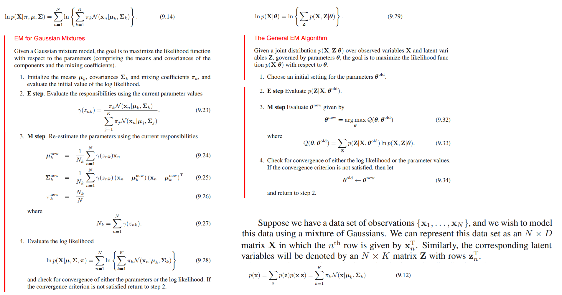
Iterative EM algorithm:
We first choose some initial values for the means, covariances, and mixing coefficients. Then we alternate between the following two updates that we shall call the E step and the M step.
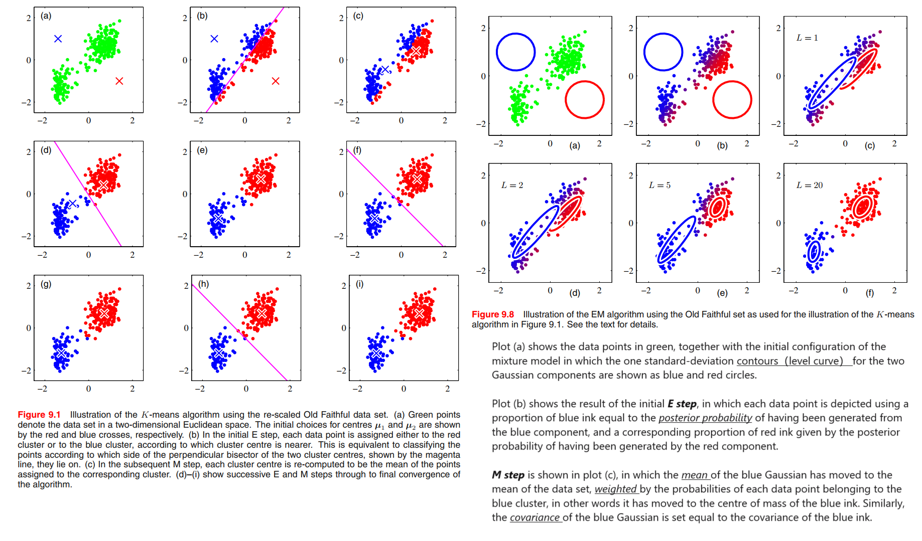
In the expectation step, or E step, we use the current values for the parameters to evaluate the posterior probabilities, or responsibilities, given by (9.13). We then use these probabilities in the maximization step, or M step, to re-estimate the means, covariances, and mixing coefficients using the results (9.17), (9.19), and (9.22).
As with gradient-based approaches for maximizing the log likelihood, techniques must be employed to avoid singularities of the likelihood function in which a Gaussian component collapses onto a particular data point.
It should be emphasized that there will generally be multiple local maxima of the log likelihood function, and that EM is not guaranteed to find the largest of these maxima.
An Alternative View of EM
The goal of the EM algorithm is to find maximum likelihood solutions for models having latent variables.
The set of all model parameters is denoted by $\pmb{\theta}$, and so the log likelihood function is given by
$$
\ln p(\pmb{X}|\pmb{\theta}) = \ln \left\{ \sum_{\pmb{Z}} p(\pmb{X,Z|\theta}) \right\}
\tag{9.29}
$$
Note that our discussion will apply equally well to continuous latent variables simply by replacing the sum over $\pmb{Z}$ with an integral.
Now suppose that, for each observation in $\pmb{X}$, we were told the corresponding value of the latent variable $\pmb{Z}$. We shall call $\left\{ \pmb{X}, \pmb{Z} \right\}$ the complete data set, and we shall refer to the actual observed data $\pmb{X}$ as incomplete, In practice, however, we are not given the complete data set $\left\{ \pmb{X}, \pmb{Z} \right\}$, but only the incomplete data $\pmb{X}$.
The likelihood function for the complete data set simply takes the form $\ln p(\pmb{X},\pmb{Z}|\pmb{\theta})$.
Our state of knowledge of the values of the latent variables in $\pmb{Z}$ is given only by the posterior distribution $p(\pmb{Z}| \pmb{X}, \pmb{\theta})$. Because we cannot use the complete-data log likelihood, we consider instead its expected value under the posterior distribution of the latent variable, which corresponds (as we shall see) to the $E$ step of the $EM$ algorithm.
In the E step, we use the current parameter values $\pmb{\theta^{old}}$ to find the posterior distribution of the latent variables given by $p(\pmb{Z}|\pmb{X}, \pmb{\theta^{old}})$. We then use this posterior distribution to find the expectation of the complete-data log likelihood evaluated for some general parameter value $\pmb{\theta}$. This expectation, denoted $E$, is given by
$$
E(\pmb{\theta, \theta^{old}}) = \sum_{\pmb{Z}} p(\pmb{Z} | \pmb{X}, \pmb{\theta^{old}}) \ln p(\pmb{X}, \pmb{Z} | \pmb{\theta})
\tag{9.30}
$$
In the M step, we determine the revised parameter estimate $\pmb{\theta^{new}}$ by maximizing this function
$$
\pmb{\theta^{new}} = \underset{\theta}{argmax} E (\pmb{\theta, \theta^{old}})
\tag{9.31}
$$
Gaussian mixtures revisited(with latent view)
Now consider the problem of maximizing the likelihood for the complete data set $\left\{ \pmb{X}, \pmb{Z} \right\}$. From (9.10) and (9.11), this likelihood function takes the form
$$
p(\pmb{X}, \pmb{Z} | \pmb{\mu}, \pmb{\Sigma}, \pmb{\pi}) = \prod_{n=1}^{N} \prod_{k=1}^{K} \pi_k^{z_{nk}} \mathcal{N}(\pmb{x_n} | \pmb{\mu_k}, \pmb{\Sigma_k})^{z_{nk}}
\tag{9.35}
$$
where $z_{nk}$ denotes the $k^{th}$ component of $\pmb{z}_n$. Taking the logarithm, we obtain
$$
\ln p(\pmb{X}, \pmb{Z} | \pmb{\mu}, \pmb{\Sigma}, \pmb{\pi}) = \sum_{n=1}^{N} \sum_{k=1}^{K} z_{nk} \left\{ \ln \pi_k + \ln \mathcal{N}(\pmb{x_n} | \pmb{\mu_k}, \pmb{\Sigma_k}) \right\}
\tag{9.36}
$$
by Lagrange multiplier as before,
$$
\pi_k = \frac{1}{N} \sum_{n=1}^{N} z_{nk}
\tag{9.37}
$$
Using (9.10) and (9.11) together with Bayes’ theorem, we see that this posterior distribution takes the form
$$
p(\pmb{Z}| \pmb{X}, \pmb{\mu}, \pmb{\Sigma}, \pmb{\pi}) \propto \prod_{n=1}^{N} \prod_{k=1}^{K} \left[\pi_k \mathcal{N}(\pmb{x_n} | \pmb{\mu_k}, \pmb{\Sigma_k})\right]^{z_{nk}}
\tag{9.38}
$$
The expected value of the indicator variable $z_{nk}$ under this posterior distribution is then given by
$$
E[z_{nk}] = \frac{\sum_{z_{nk}}z_{nk} [\pi_k \mathcal{N}(\pmb{x_n} | \pmb{\mu_k}, \pmb{\Sigma_k})]^{z_{nk}}}{\sum_{z_{nj}} [\pi_j \mathcal{N}(\pmb{x_n} | \pmb{\mu_j}, \pmb{\Sigma_j})]^{z_{nj}}}
=\frac{\pi_k \mathcal{N}(\pmb{x_n} | \pmb{\mu_k}, \pmb{\Sigma_k})}{\sum_{j=1}^{K}\pi_j \mathcal{N}(\pmb{x_n} | \pmb{\mu_j}, \pmb{\Sigma_j})} = \gamma(z_{nk})
\tag{9.39}
$$
The expected value of the complete-data log likelihood function is therefore given by
$$
E_{\pmb{Z}} [\ln p(\pmb{X}, \pmb{Z}| \pmb{\mu}, \pmb{\Sigma}, \pmb{\pi})] = \sum_{n=1}^{N} \sum_{k=1}^{K} \gamma(z_{nk}) \left\{ \ln \pi_k + \ln \mathcal{N}(\pmb{x_n} | \pmb{\mu_k}, \pmb{\Sigma_k}) \right\}
\tag{9.40}
$$
We can now proceed as follows.
E step : First we choose some initial values for the parameters $\pmb{\mu^{old}}$, $\pmb{\Sigma^{old}}$ and $\pmb{\pi^{old}}$, and use these to evaluate the responsibilities.
M step : We then keep the responsibilities fixed and maximize (9.40) with respect to $\pmb{\mu}$, $\pmb{\Sigma}$ and $\pmb{\pi}$.
This leads to closed form solutions for $\pmb{\mu^{new}}$, $\pmb{\Sigma^{new}}$ and $\pmb{\pi^{new}}$ given by (9.17), (9.19), and (9.22) as before.
This is precisely the EM algorithm for Gaussian mixtures as derived earlier.
Relation to K-means
Whereas the K-means algorithm performs a hard assignment of data points to clusters, in which each data point is associated uniquely with one cluster, the EM algorithm makes a soft assignment based on the posterior probabilities.
In fact, we can derive the K-means algorithm as a particular limit of EM for Gaussian mixtures as follows.
Mixtures of Bernoulli distributions
👉First Understanding Bernoulli distributions >>
EM for Bayesian linear regression
The EM Algorithm in General
👉First Understanding $KL$ Divergence >>
The expectation maximization algorithm, or EM algorithm, is a general technique for finding maximum likelihood solutions for probabilistic models having latent variables (Dempster et al., 1977; McLachlan and Krishnan, 1997).
Our goal is to maximize the likelihood function that is given by
$$
p(\pmb{X}|\pmb{\theta}) = \sum_{\pmb{Z}} p(\pmb{X}, \pmb{Z}|\pmb{\theta})
\tag{9.69}
$$
We shall suppose that direct optimization of $p(\pmb{X}|\pmb{\theta})$ is difficult, but that optimization of the complete-data likelihood function $p(\pmb{X}, \pmb{Z}|\pmb{\theta})$ is significantly easier.
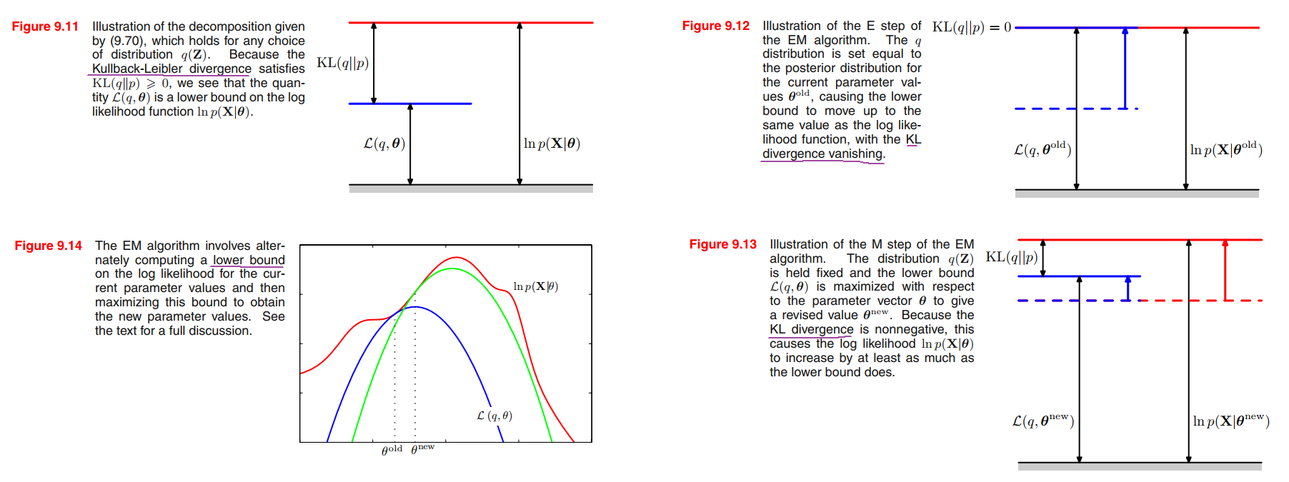
We introduce a distribution $q(\pmb{Z})$ defined over the latent variables, and we observe that, for any choice of $q(\pmb{Z})$, the following decomposition holds
$$
\ln p(\pmb{X}|\pmb{\theta}) = \mathcal{L}(q,\pmb{\theta}) + KL(q||p)
\tag{9.70}
$$
where
$$
\mathcal{L}(q,\pmb{\theta}) = \sum_{\pmb{Z}} q(\pmb{Z}) \ln \left\{ \frac{p(\pmb{X}, \pmb{Z} | \pmb{\theta})}{q(\pmb{Z})} \right\}
\tag{9.71}
$$
$$
KL(q||p) = - \sum_{\pmb{Z}} q(\pmb{Z}) \ln \left\{ \frac{p(\pmb{Z}|\pmb{X}, \pmb{\theta})}{q(\pmb{Z})} \right\}
\tag{9.72}
$$
Note that $\mathcal{L}(q, \pmb{\theta})$ is a functional of the distribution $q(\pmb{Z})$, and a function of the parameters $\pmb{\theta}$.
Proof of (9.70):