Keywords: SubSpaces, NullSpace and ColSpace, Coordinates Mapping, Dimension, Rank, Difference Equation, Markov Chains
This is the Chapter4 ReadingNotes from book Linear Algebra and its Application.
Vector Spaces and SubSpaces
A subspace of a vector space $V$ is a subset $H$ of $V$ that has three properties:
a. The zero vector of $V$ is in $H$.
b. $H$ is closed under vector addition. That is, for each $\vec{u}$ and $\vec{v}$ in $H$, the sum $\vec{u} + \vec{v}$ is in $H$.
c. $H$ is closed under multiplication by scalars. That is, for each $\vec{u}$ in $H$ and each scalar $c$, the vector $c\vec{u}$ is in $H$.
if $\vec{v_1} \cdots \vec{v_p}$ are in a vector space $V$, then Span{$\vec{v_1} \cdots \vec{v_p}$} is a subspace of $V$.
💡For Example💡:
Let $H$ be the set of all vectors of the form $(a - 3b, b - a, a, b)$, where $a$ and $b$ are arbitrary scalars. That is, let $H = \lbrace a - 3b, b - a, a, b \rbrace$, $a$ and $b$ in $R$. Show that $H$ is a subspace of $R^4$.
Proof:
Write the vectors in $H$ as column vectors. Then the arbitrary vector in $H$ has the form
$$
\begin{bmatrix}
a-3b \\ b-a \\ a \\ b
\end{bmatrix}
=
a\begin{bmatrix}
1 \\ -1 \\ 1 \\ 0
\end{bmatrix} +
b\begin{bmatrix}
-3 \\ 1 \\ 0 \\ 1
\end{bmatrix}
$$
This calculation shows that H = Span{$\vec{v_1}, \vec{v_2}$}, where $\vec{v_1}$ and $\vec{v_2}$ are the vectors indicated above. Thus $H$ is a subspace of $R^4$.
Null Spaces, Column Spaces, And Linear Transformations
The Null Space of a Matrix
The null space of an $m \times n$ matrix $A$, written as $Nul A$, is the set of all solutions of the homogeneous equation $A\vec{x} = \vec{0}$. In set notation,
$$
Nul A = \lbrace\vec{x} : \vec{x} \space in\space R^n and A\vec{x} = 0\rbrace
$$
The null space of an $m \times n$ matrix $A$ is a subspace of $R^n$.
An Explicit Description of Nul A
💡For Example💡:
Find a spanning set for the null space of the matrix
$$
A =
\begin{bmatrix}
-3 & 6 & -1 & 1 & -7\\
1 & -2 & 2 & 3 & -1\\
2 & -4 & 5 & 8 & -4
\end{bmatrix}
$$
Solution:
$$
\begin{bmatrix}
-3 & 6 & -1 & 1 & -7 & 0\\
1 & -2 & 2 & 3 & -1 & 0\\
2 & -4 & 5 & 8 & -4 & 0
\end{bmatrix}
\sim
\begin{bmatrix}
1 & -2 & 0 & -1 & 3 & 0\\
0 & 0 & 1 & 2 & -2 & 0\\
0 & 0 & 0 & 0 & 0 & 0
\end{bmatrix}
\begin{bmatrix}
x_1 \\ x_2 \\ x_3 \\x_4 \\x_5
\end{bmatrix} =
\begin{bmatrix}
2x_2+x_4-3x_5 \\ x_2 \\ -2x_4+2x_5 \\x_4 \\x_5
\end{bmatrix} =
x_2\begin{bmatrix}
2 \\ 1 \\ 0 \\ 0 \\ 0
\end{bmatrix} +
x_4\begin{bmatrix}
1 \\ 0 \\ -2 \\ 1 \\ 0
\end{bmatrix} +
x_5\begin{bmatrix}
-3 \\ 0 \\ 2 \\ 0 \\ 1
\end{bmatrix}
= x_2\vec{u} + x_4\vec{v} + x_5\vec{w}
$$
Every linear combination of $\vec{u},\vec{v},\vec{w}$ is an element of $Nul A$ and vice versa. Thus $\lbrace\vec{u},\vec{v},\vec{w}\rbrace$ is a spanning set for $Nul A$.
The Column Space of a Matrix
The column space of an $m \times n$ matrix A, written as $Col A$, is the set of all linear combinations of the columns of A. If $A = \left[\vec{a_1}, \cdots, \vec{a_n}\right]$, then
$$
ColA = Span\lbrace\vec{a_1}, \cdots, \vec{a_n}\rbrace
$$
The column space of an $m \times n$ matrix A is a subspace of $R^m$.
Note that a typical vector in $Col A$ can be written as $A\vec{x}$ for some $\vec{x}$ because the notation $A\vec{x}$ stands for a linear combination of the columns of $A$. That is,
$$
Col A = \lbrace \vec{b} : \vec{b} = A \vec{x} for \space some\space x \space in \space R^n\rbrace
$$
The Contrast Between Nul A and Col A
Contrast Between $NulA$ and $ColA$ for an $m \times n$ Matrix $A$
| $NulA$ | $ColA$ |
|---|---|
| 1. $NulA$ is a subspace of $R^n$. | 1.$ColA$ is a subspace of $R^m$. |
| 2.$NulA$ is implicitly defined; that is, you are given only a condition $A\vec{x}=\vec{0}$that vectors in $NulA$ must satisfy. | 2.$ColA$ is explicitly defined; that is, you are told how to build vectors in $ColA$. |
| 3. it takes time to find vectors in $NulA$. Row operations on $\begin{bmatrix}A & \vec{0} \end{bmatrix}$ are required. | 3. It is easy to find vectors in $ColA$. The columns of $A$ are displayed; others are formed from them |
| 4. There is no obvious relation between $NulA$ and the entries in $A$. | 4. There is an obvious relation between $ColA$ and the entries in $A$, since each column of $A$ is in $ColA$. |
| 5. A typical vector $\vec{v}$ in $NulA$ has the property that $A\vec{v} = \vec{0}$. | 5. A typical vector $\vec{v}$ in$ColA$has the property that the equation $A\vec{x} = \vec{v}$ is consistent. |
| 6. Given a specific vector $\vec{v}$, it is easy to tell if $\vec{v}$ is in $NulA$. Just compute $A\vec{v}$. | 6. Given a specific vector $\vec{v}$, it may take time to tell if $\vec{v}$ is in $ColA$. Row operations on are required. |
| 7. $NulA = \lbrace\vec{0}\rbrace$ if and only if the equation $A\vec{x} = \vec{0}$ has only the trivial solution. | 7. $ColA = R^m$ if and only if the equation $A\vec{x} = \vec{b}$ has a solution for every $\vec{b}$ in $R^m$. |
| 8. $NulA = \lbrace\vec{0}\rbrace$ if and only if the linear transformation $\vec{x} \mapsto A\vec{x}$ is one-to-one. | 8.$ColA = R^m$ if and only if the linear transformation $\vec{x} \mapsto A\vec{x}$ maps $R^n$ onto $R^m$. |
Linearly Independent Sets; Bases
An indexed set $\lbrace \vec{v_1}, \cdots, \vec{v_p} \rbrace$ of two or more vectors, with $\vec{v_1} \neq \vec{0}$, is linearly depentdent if and only if some $\vec{v_j}$(with $j > 1$) is a linear combination if the preceding vectors $\vec{v_1}, \cdots, \vec{v_{j-1}}$.
Let $H$ be a subspace of a vector space $V$. An indexed set of vectors $\beta = \lbrace \vec{b_1}, \cdots, \vec{b_p}\rbrace$ in $V$ is a basis for $H$ if
(i) $\beta$ is a linearly independent set, and
(ii) the subspace spanned by $\beta$ coincides with $H$; that is $$H = Span \lbrace \vec{b_1}, \cdots, \vec{b_p} \rbrace$$
💡For Example💡:
Let $S = \lbrace 1, t, t^2, \cdots, t^n \rbrace$. Verify that $S$ is a basis for $P_n$. This basis is called the standard basis for $P_n$.
Solution:
Certainly $S$ spans $P_n$. To show that S is linearly independent, suppose that $c_0, \cdots, c_n$ satisfy
$$
c_0 \cdot 1 + c_1 \cdot t + c_2 \cdot t^2 + \cdots + c_n \cdot t^n = \vec{0_t}\tag{2}
$$
This equality means that the polynomial on the left has the same values as the zero polynomial on the right. A fundamental theorem in algebra says that the only polynomial in $P_n$ with more than $n$ zeros is the zero polynomial. That is, equation (2) holds for all $t$ only if $c_0 = \cdots = c_n = 0$. This proves that $S$ is linearly independent and hence is a basis for $P_n$.
The Spanning Set Theorem
Let $S = \lbrace \vec{v_1}, \cdots, \vec{v_p} \rbrace$ be a set in $V$, and let $H = \lbrace \vec{v_1}, \cdots, \vec{v_p} \rbrace$.
a. If one of the vectors in $S$-say, $\vec{v_k}$- is a linear combination of the remaining vectors in $S$, then the set formed from $S$ by removing $\vec{v_k}$ still spans $H$.
b. If $H \neq \lbrace \vec{0}\rbrace$, some subset of $S$ is a basis for $H$.
Bases for Nul A and Col A
The pivot columns of a matrix A form a basis for Col A.
Two Views of a Basis
💡For Example💡:
The following three sets in $R^3$ show how a linearly independent set can be enlarged to a basis and how further enlargement destroys the linear independence of the set. Also, a spanning set can be shrunk to a basis, but further shrinking destroys the spanning property.
Linearly independent,but does not span $R^3$:
$$
\lbrace
\begin{bmatrix}
1\\0\\0
\end{bmatrix},
\begin{bmatrix}
2\\3\\0
\end{bmatrix}
\rbrace
$$
A basis for $R^3$:
$$
\lbrace
\begin{bmatrix}
1\\0\\0
\end{bmatrix},
\begin{bmatrix}
2\\3\\0
\end{bmatrix},
\begin{bmatrix}
4\\5\\6
\end{bmatrix}
\rbrace
$$
Spans $R^3$ but is linearly dependent:
$$
\lbrace
\begin{bmatrix}
1\\0\\0
\end{bmatrix},
\begin{bmatrix}
2\\3\\0
\end{bmatrix},
\begin{bmatrix}
4\\5\\6
\end{bmatrix},
\begin{bmatrix}
7\\8\\9
\end{bmatrix}
\rbrace
$$
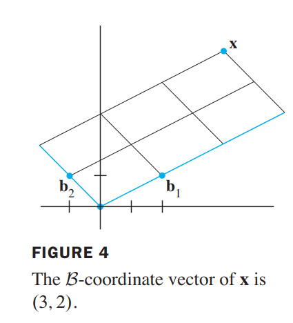
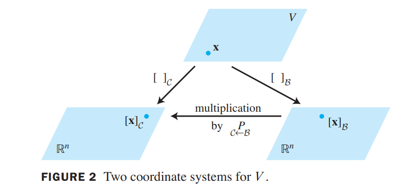
Coordinate Systems
Let $\beta = \lbrace \vec{b_1}, \cdots, \vec{b_n}\rbrace$ be a basis for a vector space $V$. Then for each $\vec{x}$ in $V$, there exists a unique set of scalars $c_1, \cdots, c_n$ such that
$$
\vec{x} = c_1\vec{b_1} + \cdots + c_n \vec{b_n}
$$
Suppose $\beta = \lbrace \vec{b_1}, \cdots, \vec{b_n}\rbrace$ is a basis for $V$ and $\vec{x}$ is in $V$. The coordinates of x relative to the basis $\beta$ (or the $\beta $-coordinates of x) are the weights $c_1, \cdots, c_n$ such that
$$
\vec{x} = c_1\vec{b_1} + \cdots + c_n\vec{b_n}
$$
If $c_1, \cdots, c_n$ are the $\beta$-coordinates of $\vec{x}$, then the vector in $R^n$
$$
[\vec{x}]_\beta =
\begin{bmatrix}
c_1 \\ \cdots \\c_n
\end{bmatrix}
$$
is the coordinate vector of $\vec{x}$ (relative to $\beta$), the mapping $\vec{x} \mapsto [\vec{x}]_\beta$ is the coordinate mapping (determined by $\beta$).
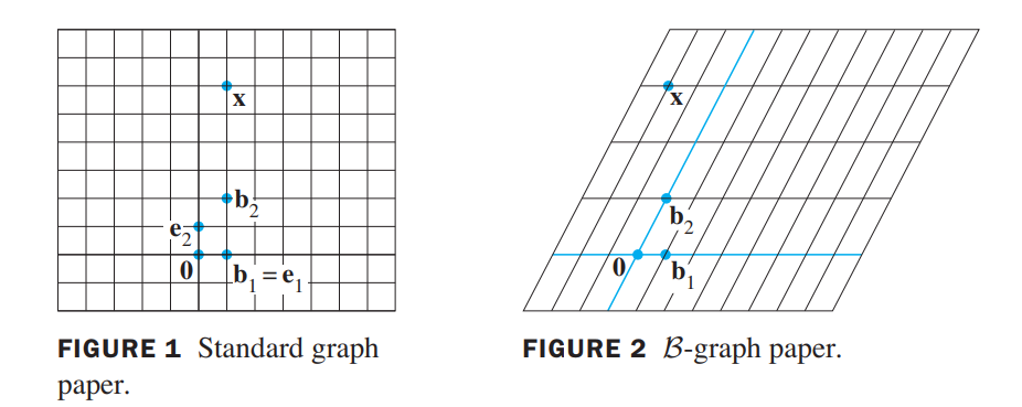
A Graphical Interpretation of Coordinates
1 unit in the $\vec{e_1}$ direction, 6 units in the $\vec{e_2}$ direction:
$$
\vec{x} =
\begin{bmatrix}
1 \\ 6
\end{bmatrix}
$$
2 units in the $\vec{b_1}$ direction, 3 units in the $\vec{b_2}$ direction:
$$
[\vec{x}]_\beta =
\begin{bmatrix}
-2 \\ 3
\end{bmatrix}
$$
Coordinates in $R^n$
💡For Example💡:
Let $\vec{b_1} = \begin{bmatrix} 2 \\ 1 \end{bmatrix}$,$\vec{b_2} = \begin{bmatrix} -1 \\ 1 \end{bmatrix}$,$\vec{x} = \begin{bmatrix} 4 \\ 5 \end{bmatrix}$, and $\beta = \lbrace \vec{b_1}, \vec{b_2}\rbrace$. Find the coordinate vector $[\vec{x}]_\beta$ of $\vec{x}$ relative to $\beta$.
Solution:
The $\beta$-coordinates $c_1, c_2$ of $\vec{x}$ satisfy
$$
c_1\begin{bmatrix}2 \\ 1\end{bmatrix} + c_2\begin{bmatrix}-1 \\ 1\end{bmatrix}
= \begin{bmatrix}4 \\ 5\end{bmatrix},
\begin{bmatrix}2 & -1 \\ 1 & 1\end{bmatrix} \begin{bmatrix}c_1 \\ c_2\end{bmatrix}
= \begin{bmatrix}4 \\ 5\end{bmatrix}
\tag{3}
$$
This equation can be solved by row operations on an augmented matrix or by using the inverse of the matrix on the left. In any case, the solution is
$$
c_1 = 3, c_2 = 2 \\
\vec{x} = 3\vec{b_1} + 2\vec{b_2}, and \space
[\vec{x}]_\beta = \begin{bmatrix}c_1 \\ c_2\end{bmatrix}
=\begin{bmatrix}3 \\ 2\end{bmatrix}
$$
The matrix in (3) changes the $\beta$ -coordinates of a vector $\vec{x}$ into the standard coordinates for $\vec{x}$. An analogous change of coordinates can be carried out in $R^n$ for a basis $\beta = \lbrace \vec{b_1}, \cdots, \vec{b_n} \rbrace$. Let
$$
P_\beta =
\begin{bmatrix}
\vec{b_1} & \vec{b_2} & \cdots & \vec{b_n}
\end{bmatrix}
$$
Then the vector equation
$$
\vec{x} = c_1\vec{b_1} + c_2\vec{b_2} + \cdots + c_n\vec{b_n}
$$
is equivalent to
$$
\vec{x} = P_\beta[\vec{x}]_\beta
$$
We call $P_\beta$ the change-of-coordinates matrix from $\beta$ to the standard basis in $R^n$. Left-multiplication by $P_\beta$ transforms the coordinate vector $[\vec{x}]_\beta$ into $\vec{x}$.
Since the columns of $P_\beta$ form a basis for $R^n$, $P_\beta$ is invertible. Left-multiplication by $P_\beta^{-1}$converts $\vec{x}$ into its $\beta$-coordinate vector:
$$
P_\beta^{-1}\vec{x} = [\vec{x}]_\beta
$$
The Coordinate Mapping
Choosing a basis $\beta = \lbrace \vec{b_1}, \cdots, \vec{b_n} \rbrace$ for a vector space $V$ introduces a coordinate system in $V$. The coordinate mapping $\vec{x} \mapsto [\vec{x}]_\beta$ connects the possibly unfamiliar space $V$ to the familiar space $R^n$:
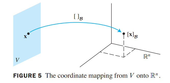
Let $\beta = \lbrace \vec{b_1}, \cdots, \vec{b_n} \rbrace$ be a basis for a vector space $V$. Then the coordinate mapping $\vec{x} \mapsto [\vec{x}]_\beta$ is a one-to-one linear transformation from $V$ onto $R^n$.
这里一定要注意,beta是向量空间V的基向量,x也是属于V空间的向量
Proof:
two typical vectors in $V$:
$$
\vec{u} = c_1\vec{b_1} + \cdots + c_n\vec{b_n},
\vec{w} = d_1\vec{b_1} + \cdots + d_n\vec{b_n}
\stackrel{addition-operation}\longrightarrow
\vec{u} + \vec{w} = (c_1 + d_1)\vec{b_1} + \cdots + (c_n + d_n)\vec{b_n}
\longrightarrow
\\
[\vec{u} + \vec{w}]_\beta =
\begin{bmatrix}
c_1 + d_1 \\
\cdots \\
c_n + d_n
\end{bmatrix} =
\begin{bmatrix}
c_1 \\
\cdots \\
c_n
\end{bmatrix} +
\begin{bmatrix}
d_1 \\
\cdots \\
d_n
\end{bmatrix} =
[\vec{u}]_\beta + [\vec{w}]_\beta
\\
常量乘法也一样性质,略过
$$
Thus the coordinate mapping also preserves scalar multiplication and hence is a linear transformation.
In general, a one-to-one linear transformation from a vector space $V$ onto a vector space$W$ is called an isomorphism from $V$ onto $W$.
💡For Example💡:
Let $\beta$ be the standard basis of the space $P_3$ of polynomials; that is, let $\beta = \lbrace \vec{1}, \vec{t}, \vec{t^2}, \vec{t^3}\rbrace$. A typical element $p$ of $P_3$ has the form:
$$
\vec{p(t)} = a_0 + a_1\vec{t} + a_2\vec{t^2} + a_3\vec{t^3}
$$
Since $\vec{p}$is already displayed as a linear combination of the standard basis vectors, we
conclude that:
$$
[\vec{p}]_\beta =
\begin{bmatrix}
a_0\\a_1\\a_2\\a_3
\end{bmatrix}
$$
Thus the coordinate mapping $\vec{p} \mapsto [\vec{p}]_\beta$is an isomorphism from$P_3$ onto $R_4$.
The Dimension of A Vector Space
If a vector space $V$ has a basis $\beta = \lbrace \vec{b_1}, \cdots, \vec{b_n}\rbrace$, then any set in $V$ containing more than $n$ vectors must be linearly dependent.
If a vector space $V$ has a basis of $n$ vectors, then every basis of $V$ must consist of exactly $n$ vectors.
If $V$ is spanned by a finite set, then $V$ is said to be finite-dimensional, and the dimension of $V$ , written as $dim V$ , is the number of vectors in a basis for $V$. The dimension of the zero vector space ${\vec{0}}$ is defined to be zero. If $V$ is not spanned by a finite set, then V is said to be infinite-dimensional.
💡For Example💡:
Find the dimension of the subspace:
$H = \lbrace \begin{bmatrix} a - 3b + 6c\\5a + 4d\\ b - 2c - d\\5d\end{bmatrix} a,b,c,d \space in R \rbrace$
Solution:
$H$ is the set of all linear combinations of the vectors:
$$
\vec{v_1} =
\begin{bmatrix}
1\\5\\0\\0
\end{bmatrix},
\vec{v_2} =
\begin{bmatrix}
-3\\0\\1\\0
\end{bmatrix},
\vec{v_3} =
\begin{bmatrix}
6\\0\\-2\\0
\end{bmatrix},
\vec{v_4} =
\begin{bmatrix}
0\\4\\-1\\5
\end{bmatrix}
$$
$\lbrace \vec{v_1}, \vec{v_2}, \vec{v_4}\rbrace$ is linearly independent and hence is a basis for $H$. Thus $dim H = 3$.
Subspaces of a Finite-Dimensional Space
Let $H$ be a subspace of a finite-dimensional vector space $V$ . Any linearly independent set in $H$ can be expanded, if necessary, to a basis for $H$ . Also, $H$ is finite-dimensional and
$$
dim H \leqslant dim V
$$
The Dimensions of $Nul A$ and $Col A$
The dimension of $Nul A$ is the number of free variables in the equation $A\vec{x} = \vec{0}$, and the dimension of $Col A$ is the number of pivot columns in $A$.
💡For Example💡:
Find the dimensions of the null space and the column space of $A = \begin{bmatrix}-3 & 6 & -1 & 1 & -7\\1 & -2 & 2 & 3 & -1\\2 & -4 & 5 & 8 & -4\end{bmatrix}$
$$
\begin{bmatrix}
1 & -2 & 2 & 3 & -1 & 0\\
0 & 0 & 1 & 2 & -2 & 0\\
0 & 0 & 0 & 0 & 0 & 0
\end{bmatrix}
\
x_2, x_4, x_5: free\space variables\\
\longrightarrow dimNulA = 3, dimColA = 2.
$$
Rank
The Row Space
If two matrices $A$ and $B$ are row equivalent, then their row spaces are the same. If $B$ is in echelon form, the nonzero rows of $B$ form a basis for the row space of $A$ as well as for that of $B$.
💡For Example💡:
Find bases for the row space, the column space, and the null space of the matrix $\begin{bmatrix}-2 & -5 & 8 & 0 & -17\\1 & 3 & -5 & 1 & 5\\3 & 11 & -19 & 7 & 1\\1 & 7 & -13 & 5 & -3\end{bmatrix}$.
$$
A \sim B =
\begin{bmatrix}
1 & 3 & -5 & 1 & 5\\
0 & 1 & -2 & 2 & -7\\
0 & 0 & 0 & -4 & 20\\
0 & 0 & 0 & 0 & 0
\end{bmatrix}
\sim C =
\begin{bmatrix}
1 & 0 & 1 & 0 & 1\\
0 & 1 & -2 & 0 & 3\\
0 & 0 & 0 & 1 & -5\\
0 & 0 & 0 & 0 & 0
\end{bmatrix}
\\
(只需看前几行非零)
Basis-for-RowA:\lbrace(1, 3, 5, 1, 5),(0, 1, 2, 2, 7),(0, 0, 0, 4, 20)\rbrace
\\
(要看pivot \space columns)
Basis-for-ColA:\lbrace
\begin{bmatrix}-2\\ 1\\ 3\\ 1\end{bmatrix},
\begin{bmatrix}-5\\ 3\\ 11\\ 7\end{bmatrix},
\begin{bmatrix}0\\ 1\\ 7\\ 5\end{bmatrix}\rbrace
\\
(求解,有两个自由变量)
Basis-for-NullA:\lbrace
\begin{bmatrix}-1\\ 2\\ 1\\ 0\\ 0\end{bmatrix},
\begin{bmatrix}-1\\ -3\\ 0\\ 5\\ 1\end{bmatrix}\rbrace
$$
The Rank Theorem
The rank of $A$ is the dimension of the column space of $A$.
The dimensions of the column space and the row space of an $m \times n$ matrix $A$ are equal. This common dimension, the rank of $A$, also equals the number of pivot positions in $A$ and satisfies the equation
$$
rank A + dim NullA = n
\\
其实就是:
\\
\lbrace number-of-pivot-columns\rbrace +
\lbrace number-of-nonpivot-columns\rbrace =
\lbrace number-of-columns\rbrace
$$
Applications to Systems of Equations
💡For Example💡:
A scientist has found two solutions to a homogeneous system of 40 equations in 42 variables. The two solutions are not multiples, and all other solutions can be constructed by adding together appropriate multiples of these two solutions. Can the scientist be certain that an associated nonhomogeneous system (with the same coefficients) has a solution?
Solution:
Yes. Let $A$ be the $40 \times 42$ coefficient matrix of the system. The given information implies that the two solutions are linearly independent and span $Nul A$.
So $dim Nul A = 2$. By the Rank Theorem, $dim Col A = 42 - 2 = 40$. Since $R^{40}$ is the only subspace of $R^{40}$ whose dimension is $40$, $Col A$ must be all of $R^{40}$. This means that every nonhomogeneous equation $Ax = b$ has a solution.
Rank and the Invertible Matrix Theorem
The Invertible Matrix Theorem
Let $A$ be an $n \times n$ matrix. Then the following statements are each equivalent to the statement that $A$ is an invertible matrix.
m.The columns of $A$ form a basis of $R^n$.
n. $Col A = R^n$
o. $dim Col A = n$
p. $rank A = n$
q. $Nul A = \lbrace 0 \rbrace $
r. $dim Nul A = 0$
Change of Basis
💡For Example💡:
Consider two bases $\beta = \lbrace \vec{b_1}, \vec{b_2}\rbrace$ and $\gamma = \lbrace \vec{c_1}, \vec{c_2}\rbrace$ for a vector space $V$, such that
$$
\vec{b_1} = 4 \vec{c_1} + \vec{c_2} \space and \space \vec{b_2} = -6 \vec{c_1} + \vec{c_2}\tag{1}
$$
Suppose
$$
\vec{x} = 3\vec{b_1} + \vec{b_2}
\tag{2}
$$
That is, suppose $[\vec{x}]_\beta = \begin{bmatrix}3\\1\end{bmatrix}$. Find $[\vec{x}]_\gamma$.
Solution:
Apply the coordinate mapping determined by $\gamma$ to $\vec{x}$ in (2). Since the coordinate mapping is a linear transformation.
$$
[\vec{x}]_\gamma = [3\vec{b_1}+\vec{b_2}]_\gamma
= 3[\vec{b_1}]_\gamma+[\vec{b_2}]_\gamma
$$
We can write this vector equation as a matrix equation, using the vectors in the linear combination as the columns of a matrix:
$$
[\vec{x}]_\gamma =
\begin{bmatrix}
[\vec{b_1}]_\gamma & [\vec{b_2}]_\gamma
\end{bmatrix}
\begin{bmatrix}
3\\ 1
\end{bmatrix}
$$
From (1),
$$
[\vec{b_1}]_\gamma =
\begin{bmatrix}
4\\ 1
\end{bmatrix},
[\vec{b_2}]_\gamma =
\begin{bmatrix}
-6\\ 1
\end{bmatrix}
$$
Thus,
$$
[\vec{x}]_\gamma =
\begin{bmatrix}
4 & -6\\
1 & 1
\end{bmatrix}
\begin{bmatrix}
3\\ 1
\end{bmatrix}=
\begin{bmatrix}
6\\ 4
\end{bmatrix}
$$
Let $\beta = \lbrace \vec{b_1}, \cdots, \vec{b_n}\rbrace$ and $\gamma = \lbrace \vec{c_1}, \cdots, \vec{c_n}\rbrace$ be bases of a vector space $V$. Then there is a unique $n \times n$ matrix $\gamma \stackrel{P}\leftarrow \beta$ such that
$$
[\vec{x}]_\gamma =\gamma \stackrel{P}\leftarrow \beta [\vec{x}]_\beta
$$
The columns of $\gamma \stackrel{P}\leftarrow \beta$ are the $\gamma$-coordinate vectors of the vectors in the basis $\beta$. That is,
$$
\gamma \stackrel{P}\leftarrow \beta =
\begin{bmatrix}
[\vec{b_1}]\gamma & [\vec{b_2}]\gamma \cdots [\vec{b_n}]\gamma
\end{bmatrix}
$$
$\gamma \stackrel{P}\leftarrow \beta$ is called the change-of-coordinates matrix from $\beta$ to $\gamma$.
Multiplication by $\gamma \stackrel{P}\leftarrow \beta$ converts $\beta$-coordinates into $\gamma$-coordinates.
Change of Basis in $R^n$
💡For Example💡:
Let $\vec{b_1} = \begin{bmatrix}-9\\1\end{bmatrix}$,$\vec{b_2} = \begin{bmatrix}-5\\-1\end{bmatrix}$,$\vec{c_1} = \begin{bmatrix}1\\-4\end{bmatrix}$,$\vec{c_2} = \begin{bmatrix}3\\-5\end{bmatrix}$, and consider the bases for $R^2$ given by $\beta = \lbrace \vec{b_1}, \vec{b_2}\rbrace$ and $\gamma = \lbrace \vec{c_1}, \vec{c_2}\rbrace$. Find the change-of-coordinates matrix from $\beta$ to $\gamma$.
Solution:
The matrix $\gamma \stackrel{P}\leftarrow \beta$ involves the $\gamma$-coordinate vectors of $\vec{b_1}$ and $\vec{b_2}$. Let $[\vec{b_1}_\gamma] = \begin{bmatrix}x_1\\x_2\end{bmatrix}$ and $[\vec{b_2}_\gamma] = \begin{bmatrix}y_1\\y_2\end{bmatrix}$. Then, by definition,
$$
\begin{bmatrix}\vec{c_1} & \vec{c_2}\end{bmatrix}
\begin{bmatrix}\vec{x_1} \\ \vec{x_2}\end{bmatrix}
=\vec{b_1} \space and \space
\begin{bmatrix}\vec{c_1} & \vec{c_2}\end{bmatrix}
\begin{bmatrix}\vec{y_1} \\ \vec{y_2}\end{bmatrix}
=\vec{b_2}
$$
To solve both systems simultaneously, augment the coefficient matrix with $\vec{b1}$ and $\vec{b2}$, and row reduce:
$$
\left[
\begin{array}{cc|c}
\vec{c_1} & \vec{c_2} & \vec{b_1} & \vec{b_2}\end{array}
\right] =
\left[
\begin{array}{cc|cc}
-1 & 3 & -9 & -5 \\
-4 & -5 & 1 & -1\end{array}
\right]
\sim
\left[
\begin{array}{cc|cc}
1 & 0 & 6 & 4 \\
0 & 1 & -5 & -3\end{array}
\right]
$$
Thus
$$
[\vec{b_1}]_\gamma =
\begin{bmatrix}
6 \\ -5
\end{bmatrix}
\space and \space
[\vec{b_2}]_\gamma =
\begin{bmatrix}
4 \\ -3
\end{bmatrix}
$$
The desired change-of-coordinates matrix is therefore
$$
\gamma \stackrel{P}\leftarrow \beta
=
\begin{bmatrix}
[\vec{b_1}]_\gamma & [\vec{b_2}]_\gamma
\end{bmatrix}
=
\begin{bmatrix}
6 & 4 \\ -5 & -3
\end{bmatrix}
$$
An analogous procedure works for finding the change-of-coordinates matrix between any two bases in $R^n$:
$$
\left[
\begin{array}{cc|c}
\vec{c_1} & \vec{c_2} & \vec{b_1} & \vec{b_2}\end{array}
\right]
\sim
\left[
\begin{array}{c|c}
I & \gamma \stackrel{P}\leftarrow \beta
\end{array}
\right]
$$
the change-ofcoordinate matrices $P_\beta$ and $P_\gamma$ that convert $\beta$-coordinates and $\gamma$-coordinates, respectively, into standard coordinates.
$$
P_\beta[\vec{x}]_\beta = \vec{x}, \space
P_\gamma[\vec{x}]_\gamma = \vec{x}, \space and \space
[\vec{x}]_\gamma = P_\gamma^{-1}\vec{x}
$$
Thus,
$$
[\vec{x}]_\gamma = P_\gamma^{-1}\vec{x} = P_\gamma^{-1}P_\beta[\vec{x}]_\beta
\\
\Rightarrow
\\
\gamma \stackrel{P}\leftarrow \beta = P_\gamma^{-1}P_\beta
$$
👉More about Coordinates Space and Transformations in Graphics >>
Applications to Difference Equation差分方程
Linear Independence in the Space $S$ of Signals
we consider a set of only three signals in $S$, say, $\lbrace u_k \rbrace,\lbrace v_k \rbrace,\lbrace w_k \rbrace$.They are linearly independent precisely when the equation
$$
c_1 u_k + c_2 v_k + c_3 w_k = 0 for\space all \space k\tag{1}
$$
implies that $c1 = 0, c2 = 0, c3 = 0$.Then equation (1) holds for any three consecutive values of $k$, say, $k, k + 1, \space and \space k + 2$.
Hence $c1, c2, c3$ satisfy
$$
\begin{bmatrix}
u_k & v_k & w_k\\
u_{k+1} & v_{k+1} & w_{k+1}\\
u_{k+2} & v_{k+2} & w_{k+2}
\end{bmatrix}
\begin{bmatrix}
c_1\\c_2\\c_3\\
\end{bmatrix}=
\begin{bmatrix}
0\\0\\0
\end{bmatrix}\tag{2}
$$
The coefficient matrix in this system is called the Casorati matrix of the signals, and the determinant of the matrix is called the Casoratian of $u_k, v_k, w_k$. If the Casorati matrix is invertible for at least one value of k, then (2) will imply that $c1 = c2 = c3 = 0$, which will prove that the three signals are linearly independent.
💡For Example💡:
Verify that $1^k, (-2)^k, and \space 3^k$ are linearly independent signals.
Solution:
The Casorati matrix is:
$$
\begin{bmatrix}
1^k & (-2)^k & 3^k\\
1^{k+1} & (-2){k+1} & 3^{k+1}\\
1^{k+2} & (-2)^{k+2} & 3^{k+2}
\end{bmatrix}
$$
The Casorati matrix is invertible for $k = 0$. So $1^k, (-2)^k, 3^k$ are linearly independent.
Linear Difference Equations(线性差分方程)
Given scalars $a_0,\cdots, a_n$, with $a_0$ and $a_n$ nonzero, and given a signal $\lbrace z_k \rbrace$, the equation
$$
a_0y_{k+n} + a_1y_{k+n-1} + \cdots + a_ny_k = z_k for\space all\space k \tag{3}
$$
is called a linear difference equation (or linear recurrence relation) of order $n$. For simplicity, $a_0$ is often taken equal to 1. If $\lbrace z_k \rbrace$ is the zero sequence, the equation is homogeneous; otherwise, the equation is nonhomogeneous.
在第一章节的笔记中,有提一嘴Fibonacci数列是差分方程,具体形式如下,
为什么看起来是差分方程的定义不太一样?(接着看下面的内容)
$$
\vec{x_{k+1}} = A\vec{x_k}, k = 0,1,2,…\tag{5}
$$
$$
Fibonacci\\
f(0) = 0, f(1) = 1\\
f(n) = f(n-1) + f(n-2), n > 1
$$
建立矩阵方程如下:
$$
let \space F(n) = \begin{bmatrix}f(n) \\ f(n+1)\end{bmatrix}\\
AF(n) = F(n+1)\rightarrow
A\begin{bmatrix}f(n) \\ f(n+1)\end{bmatrix} =
\begin{bmatrix}f(n+1) \\ f(n+2)\end{bmatrix}
\\
\rightarrow
A = \begin{bmatrix}0 & 1 \\ 1 & 1\end{bmatrix}
\\
\Rightarrow
F(n) = A^nF(0), F(0) = \begin{bmatrix}0 \\ 1\end{bmatrix}
$$
💡For Example💡:
In digital signal processing, a difference equation such as (3) describes a linear filter, and $a_0,\cdots, a_n$ are called the filter coefficients. If $\lbrace y_k \rbrace$ is treated as the input and $\lbrace z_k \rbrace$ as the output, then the solutions of the associated homogeneous equation are the signals that are filtered out and transformed into the zero signal. Let us feed two different signals into the filter
$$
0.35y_{k+2} + 0.5y_{k+1} + 0.35y_k = z_k
$$
Here $0.35$ is an abbreviation for $\sqrt2/4$. The first signal is created by sampling the continuous signal $y = \cos(\pi t / 4)$at integer values of $t$, as in Figure3(a). The discrete signal is
$$
\lbrace y_k\rbrace = \lbrace \cdots, \cos(0), \cos(\pi/4), cos(2\pi/4), cos(3\pi/4), \cdots\rbrace
$$
For simplicity, write $\pm0.7$ in place of $\pm\sqrt2/2$, so that
$$
\lbrace y_k\rbrace = \lbrace \cdots, 1, 0.7, 0, -0.7,-1,-0.7,0,0.7,1,0.7,0 \cdots\rbrace
$$
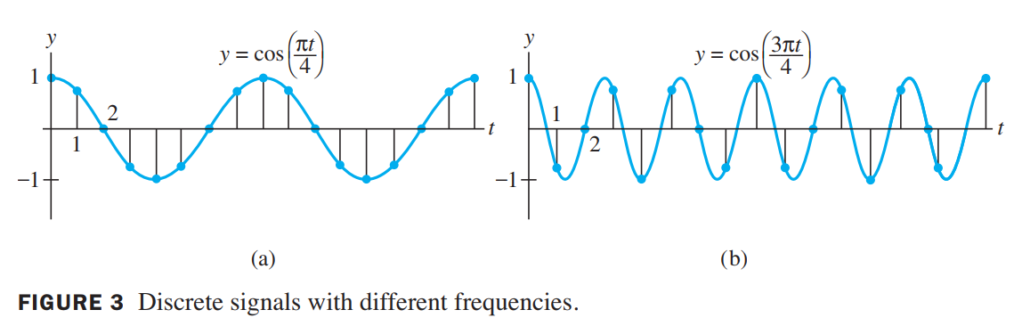
Table 1 shows a calculation of the output sequence $\lbrace z_k \rbrace$, where $0.35\cdot0.7$ is an abbreviation for $(\sqrt2/4)(\sqrt2/2)=0.25$. The output is $\lbrace y_k\rbrace$, shifted by one term.
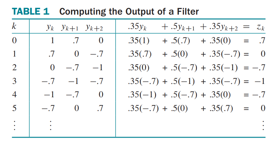
A different input signal is produced from the higher frequency signal $y = \cos(3\pi/4)$, shown in Figure 3(b). Sampling at the same rate as before produces a new input sequence:
$$
\lbrace w_k\rbrace = \lbrace \cdots, 1, -0.7, 0, 0.7, -1, 0.7, 0 \cdots\rbrace
$$
When $\lbrace w_k\rbrace$ is fed into the filter, the output is the zero sequence. The filter, called a low-pass filter(低通滤波器), lets $\lbrace y_k \rbrace$ pass through, but stops the higher frequency $\lbrace w_k \rbrace$.
In many applications, a sequence $\lbrace z_k \rbrace$ is specified for the right side of a difference equation (3), and a $\lbrace y_k \rbrace$ that satisfies (3) is called a solution of the equation. The next example shows how to find solutions for a homogeneous equation. (比如机器学习就类似于如此,给定输入和输出,学习最优权重)
💡For Example💡:
Solutions of a homogeneous difference equation often have the form $y_k = r^k$ for some $r$. Find some solutions of the equation
$$
y_{k+3} - 2y_{k+2} - 5y_{k+1} + 6y_k = 0 , for\space all\space k
$$
Solution:
Substitute $r^k$ for $y_k$ in the equation and factor the left side:
$$
r^{k+3} - 2r^{k+2} - 5r^{k+1} + 6r^{k} = 0
\rightarrow
r^k(r-1)(r+2)(r-3) = 0
$$
Thus, $(1)^k, (-2)^k, (3)^k$ are all solutions.
In general, a nonzero signal $r^k$ satisfies the homogeneous difference equation
$$
y_{k+n} + a_1y_{k+n-1} + \cdots + a_ny_k = 0 for\space all\space k
$$
if and only if $r$ is a root of the auxiliary equation(辅助方程)
$$
r^n + a_1r^{n-1} + \cdots + a_{n-1}r + a_n = 0
$$
Solution Sets of Linear Difference Equations
if $a_n \neq 0$ and if $\lbrace z_k \rbrace$ is given, the equation
$$
y_{k+n} + a_1y_{k+n-1} + \cdots + a_{n-1}y_{k+1} + a_ny_k = z_k, for\space all\space k
$$
has a unique solution whenever $y_0, \cdots, y_{n-1}$ are specified.
The set $H$ of all solutions of the nth-order homogeneous linear difference equation
$$
y_{k+n} + a_1y_{k+n-1} + \cdots + a_{n-1}y_{k+1} + a_ny_k = 0, for\space all\space k
$$
is an $n$-dimensional vector space.
Nonhomogeneous Equations(非齐次差分方程)
The general solution of the nonhomogeneous difference equation
$$
y_{k+n} + a_1y_{k+n-1} + \cdots + a_{n-1}y_{k+1} + a_ny_k = z_k, for\space all\space k
$$
💡For Example💡:
Verify that the signal $y_k = k^2$ satisfies the difference equation
$$
y_{k+2} - 4y_{k+1} + 3y_k = -4k, for\space all\space k
\tag{12}
$$
Then find a description of all solutions of this equation.
Solution:
Substitute $k^2$ for $y_k$ on the left side of (12):
$$
(k+2)^2-4(k+1)^2+3k^2 = -4k
$$
so $k^2$is indeed a solution of (12). The next step is to solve the homogeneous equation
$$
y_{k+2} - 4y_{k+1} + 3y_k = 0, for\space all\space k
\tag{13}
$$
The auxiliary equation is
$$
r^2 -4r + 3 = (r-1)(r+3) = 0
$$
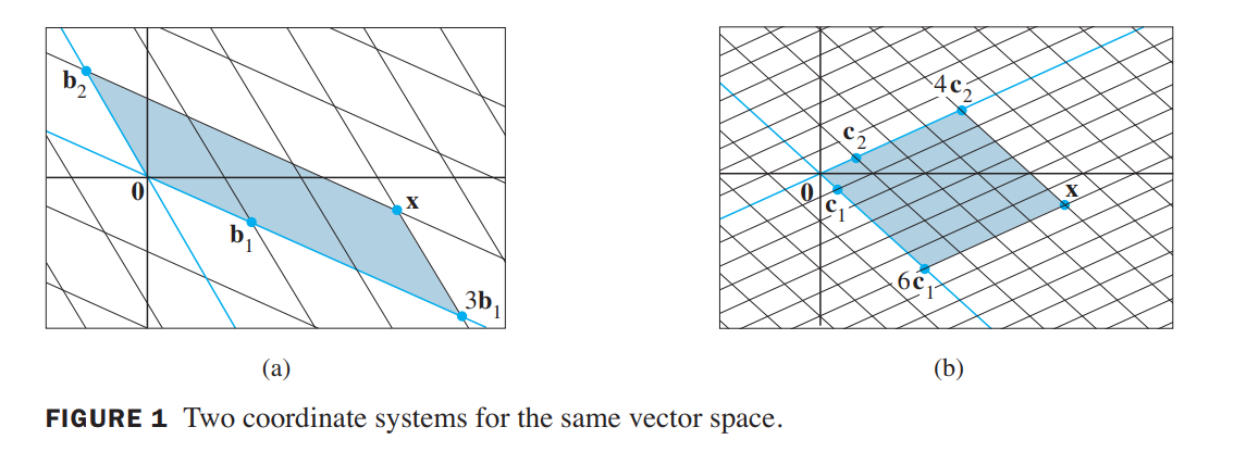
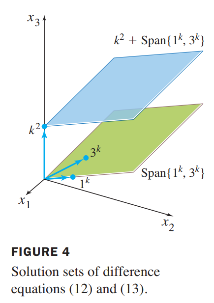
The roots are $r = 1,3$.So two solutions of the homogeneous difference equation are $1^k$ and $3^k$. They are obviously not multiples of each other, so they are linearly independent signals. the solution space is two-dimensional, so 3k and 1k form a basis for the set of solutions of equation (13).Translating that set by a particular solution of the nonhomogeneous equation (12), we obtain the general solution of (12):
$$
k^2 + c_1 1^k + c_2 3^k, or \space k^2 + c_1 + c_23^k
$$
Figure 4 gives a geometric visualization of the two solution sets. Each point in the figure corresponds to one signal in S.
Reduction to Systems of First-Order Equations(约简到一阶方程组)
接下来可以解释Fibonacci数列是差分方程
$$
AF(n) = F(n+1)\rightarrow
A\begin{bmatrix}f(n)\\f(n+1)\end{bmatrix} =
\begin{bmatrix}f(n+1)\\f(n+2)\end{bmatrix}
\
$$
A modern way to study a homogeneous $nth$-order linear difference equation is to replace it by an equivalent system of first-order difference equations, written in the form
$$
\vec{x_{k+1}} = A\vec{x_{k}}, for \space all\space k
$$
where the vectors $\vec{x_{k}}$ are in $R^n$ and $A$ is an $n \times n$ matrix.
💡For Example💡:
Write the following difference equation as a first-order system:
$$
y_{k+3} - 2y_{k+2} - 5y_{k+1} + 6y_k = 0, for \space all\space k
$$
Solution:
for each k, set
$$
\vec{x_k} =
\begin{bmatrix}
y_k\\y_{k+1}\\y_{k+2}
\end{bmatrix}
$$
The difference equation says that $y_{k+3} - 2y_{k+2} - 5y_{k+1} + 6y_k = 0$, so
$$
\vec{x_{k+1}} =
\begin{bmatrix}
y_{k+1} \\ y_{k+2} \\ y_{k+3}
\end{bmatrix} =
\begin{bmatrix}
0 + y_{k+1} + 0\\
0 + 0 + y_{k+2}\\
-6y_k + 5y_{k+1} + 2y_{k+2}
\end{bmatrix} =
\begin{bmatrix}
0 & 1 & 0\\
0 & 0 & 1\\
-6 & 5 & 2
\end{bmatrix}
\begin{bmatrix}
y_{k}\\y_{k+1}\\y_{k+2}
\end{bmatrix}
$$
That is,
$$
\vec{x_{k+1}} = A\vec{x_{k}}, for \space all\space k , where
A =
\begin{bmatrix}
0 & 1 & 0\\
0 & 0 & 1\\
-6 & 5 & 2
\end{bmatrix}
$$
In general, the equation
$$
y_{k+n} + a_1y_{k+n-1} + \cdots + a_{n-1}y_{k+1} + a_ny_k = 0, for\space all\space k
$$
can be written as $\vec{x_{k+1}} = A\vec{x_{k}}, for \space all\space k$, where
$$
\vec{x_{k}} = \begin{bmatrix}
y_{k}\\ y_{k+1} \\ \cdots \\ y_{k+n-1} \end{bmatrix},
A = \begin{bmatrix}
0 & 1 & 0 & \cdots & 0\\
0 & 0 & 1 & \cdots & 0\\
\cdots\\
0 & 0 & 0 & \cdots & 1\\
-a_n & -a_{n-1} & -a_{n-2} & \cdots & -a_1
\end{bmatrix}
$$
Applications to Markov Chains
For example, if the population of a city and its suburbs were measured each year, then a vector such as
$$
\vec{x_0} =
\begin{bmatrix}
0.60\\0.40
\end{bmatrix}
\tag{1}
$$
could indicate that 60% of the population lives in the city and 40% in the suburbs. The decimals in $\vec{x_0}$ add up to 1 because they account for the entire population of the region.Percentages are more convenient for our purposes here than population totals.
A vector with nonnegative entries that add up to 1 is called a probability vector(概率向量). A stochastic matrix(随机矩阵) is a square matrix whose columns are probability vectors. A Markov chain(马尔科夫链) is a sequence of probability vectors $\vec{x_0}, \vec{x_1}, \vec{x_2}$ together with a stochastic matrix $P$ , such that
$$
\vec{x_1} = P\vec{x_0}, \vec{x_2} = P\vec{x_1}, \vec{x_3} = P\vec{x_2}, \cdots
\\
\longrightarrow
\vec{x_{k+1}} = P\vec{x_k}
$$
$\vec{x_k}$ is often called a state vector(状态向量).
Predicting the Distant Future
💡For Example💡:
Let $P = \begin{bmatrix}0.5 & 0.2 & 0.3\\0.3 & 0.8 & 0.3\\0.2 & 0 & 0.4\end{bmatrix}$ and $\vec{x_0} = \begin{bmatrix}1\\0\\0\end{bmatrix}$. Consider a system whose state is described by the Markov chain $\vec{x_{k+1}} = P\vec{x_{k}}, for k = 0,1,\cdots$ What happens to the system as time passes? Compute the state vectors $\vec{x_1},\cdots, \vec{x_{15}}$to find out.
Solution:
$$
\vec{x_1} = P\vec{x_0} = \begin{bmatrix}0.5\\0.3\\0.2\end{bmatrix},\\
\\
\cdots
\\
\vec{x_{14}} = P\vec{x_{13}} = \begin{bmatrix}0.3001\\0.59996\\0.10002\end{bmatrix},\\
\vec{x_{15}} = P\vec{x_{14}} = \begin{bmatrix}0.3001\\0.59998\\0.10001\end{bmatrix}
$$
These vectors seem to be approaching $\vec{q} = \begin{bmatrix}0.3\\0.6\\0.1\end{bmatrix}$The probabilities are hardly changing from one value of $k$ to the next.
$$
P\vec{q} = \begin{bmatrix}0.5 & 0.2 & 0.3\\0.3 & 0.8 & 0.3\\0.2 & 0 & 0.4\end{bmatrix}
\begin{bmatrix}0.3\\0.6\\0.1\end{bmatrix}
=\begin{bmatrix}0.3\\0.6\\0.1\end{bmatrix}=\vec{q}
$$
When the system is in state $q$, there is no change in the system from one measurement to the next.
Steady-State Vectors
If $P$ is a stochastic matrix, then a steady-state vector (or equilibrium vector(平衡向量)) for $P$ is a probability vector $\vec{q}$ such that
$$
P\vec{q} = \vec{q}
$$
💡For Example💡:
Let $P = \begin{bmatrix} 0.6 & 0.3 \\ 0.4 & 0.7\end{bmatrix}$. Find a steady-state vector for $P$.
Solution:
$$
P\vec{x} = \vec{x}\rightarrow (P-I)\vec{x} = \vec{0}\
\longrightarrow
\begin{bmatrix}
-0.4 & 0.3 & 0 \\
0.4 & -0.3 & 0
\end{bmatrix}
\sim
\begin{bmatrix}
1 & -3/4 & 0 \\
0 & 0 & 0
\end{bmatrix}
$$
$$
\vec{x} = x_2\begin{bmatrix}3/4 \\ 1\end{bmatrix}
$$
Obviously, One obvious choice is $\begin{bmatrix}3/4 \\ 1\end{bmatrix}$,but a better choice with no fractions is $\vec{w} = \begin{bmatrix}3 \\ 4\end{bmatrix}, (x_2 = 4)$, since every solution is a multiple of the solution$\vec{w}$ above. Divide $\vec{w}$ by the sum of its entries and obtain
$$
\vec{q} = \begin{bmatrix}3/7 \\ 4/7\end{bmatrix}
$$
if $P$ is an $n\times n$ regular stochastic matrix, then $P$ has a unique steady-state vector $\vec{q}$. Further, if $\vec{x_0}$ is any initial state and $\vec{x_{k+1}} = P \vec{x_k}$, then the Markov chain $\vec{x_k}$ converges to $\vec{q}$ as $k \rightarrow \infty$.
Also, $\vec{q}$ is the eigenvector of $P$. See C5 ReadingNotes.

