Algebra-C5-EigenValues-And-EigenVectors

Keywords: EigenVectors, Diagonalization, Characteristic Equation, Quaternion, Differential Equation

This is the Chapter5 ReadingNotes from book Linear Algebra and its Application.

EigenVectors And EigenValues

An eigenvector of an $n \times n$ matrix $A$ is a nonzero vector $\vec{x}$ such that $A\vec{x} = \lambda\vec{x}$ for some scalar $\lambda$.
A scalar $\lambda$ is called an eigenvalue of $A$ if there is a nontrivial solution $\vec{x}$ of $A\vec{x} = \lambda\vec{x}$, such an $x$ is called an eigenvector corresponding to $\lambda$.

💡For Example💡:

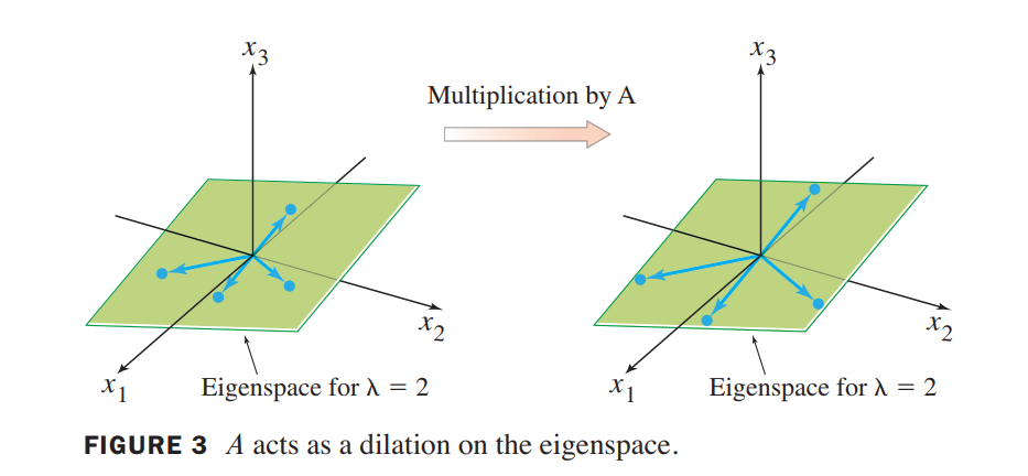
Let A = $\begin{bmatrix}4 & -1 & 6\\ 2 & 1 & 6\\ 2 & -1 & 8 \end{bmatrix}$.An eigenvalue of $A$ is 2. Find a basis for the corresponding eigenspace.

$$
A\vec{x} = 2\vec{x}
\rightarrow
(A - 2I)\vec{x} = \vec{0}
$$
$$
\begin{bmatrix}
2 & -1 & 6 & 0\\
2 & -1 & 6 & 0\\
2 & -1 & 6 & 0
\end{bmatrix}
\sim
\begin{bmatrix}
2 & -1 & 6 & 0\\
0 & 0 & 0 & 0\\
0 & 0 & 0 & 0
\end{bmatrix}
$$
general solution is:
$$
\begin{bmatrix}
x_1\\x_2\\x_3
\end{bmatrix} =
x_2\begin{bmatrix}
1/2\\1\\0
\end{bmatrix} +
x_3\begin{bmatrix}
-3\\0\\1
\end{bmatrix},
x_2 and x_3 free
$$

The eigenspace, shown in Figure 3, is a two-dimensional subspace of $R^3$. A basis is
$$
\lbrace
\begin{bmatrix}
1\\2\\0
\end{bmatrix}
\begin{bmatrix}
-3\\0\\1
\end{bmatrix}
\rbrace
$$

个人理解就是所有特征向量组成的空间就是特征空间

The eigenvalues of a triangular matrix are the entries on its main diagonal.
Let
$$
A = \begin{bmatrix}
3 & 6 & -8\\
0 & 0 & 6\\
0 & 0 & 2
\end{bmatrix},
B = \begin{bmatrix}
4 & 0 & 0\\
-2 & 1 & 0\\
5 & 3 & 4
\end{bmatrix}
$$
The eigenvalues of $A$ are $3, 0, 2$. The eigenvalues of $B$ are $4, 1$.

If $\vec{v_1},\cdots, \vec{v_r}$ are eigenvectors that correspond to distinct eigenvalues $\lambda_1, \cdots, \lambda_2$ of an $n \times n$ matrix $A$, then the set $\lbrace \vec{v_1}, \cdots , \vec{v_r}\rbrace$ is linearly independent.

Eigenvectors and Difference Equations (差分方程)

This section concludes by showing how to construct solutions of the first-order difference equation discussed in the chapter introductory example:

$$
\vec{x_{k+1}} = A\vec{x_{k}}\tag{8}
$$

If A is an $n \times n$ matrix, then (8) is a recursive description of a sequence $\lbrace \vec{x_k}\rbrace$ in $R^n$. A solution of (8) is an explicit description of $\lbrace \vec{x_k}\rbrace$ whose formula for each $\vec{x_k}$ does not depend directly on $A$ or on the preceding terms in the sequence other than the initial term $\vec{x_0}$.

The simplest way to build a solution of (8) is to take an eigenvector $\vec{x_0}$ and its corresponding eigenvalue $\lambda$and let

$$
\vec{x_k} = \lambda ^k \vec{x_0}
$$

This sequence is a solution because

$$
\begin{aligned}
A\vec{x_k} &= A(\lambda ^k \vec{x_0})\\
&=\lambda ^k A\vec{x_0} \\
&= \lambda ^k (\lambda\vec{x_0})\\
&=\vec{x_{k+1}}
\end{aligned}
$$

The Characteristic Equation（特征方程）

💡For Example💡:

Find the eigenvalues of $A = \begin{bmatrix}2 & 3 \\ 3 & -6 \end{bmatrix}$.

Solution:

We must find all scalars $\lambda$ such that the matrix equation
$$
(A - \lambda I)\vec{x} = \vec{0}
$$
has a nontrivial solution（非零解）. This problem is equivalent to finding all$\lambda$such that the matrix $A - \lambda I$ is not invertible（不可逆）, where

$$
A - \lambda I =
\begin{bmatrix}
2 - \lambda & 3\\
3 & -6-\lambda
\end{bmatrix}
\longrightarrow
det(A - \lambda I) = (\lambda - 3)(\lambda + 7) = 0
$$
so the eigenvalues of $A$ are 3 and -7.

Determinants

Let $A$ be an $n\times n$ matrix. Then A is invertible if and only if:
s. The number $0$ is not an eigenvalue of $A$.
t. The determinant of $A$ is not zero.

Let $A$ and $B$ be $n \times n$ matrices.
a. $A$ is invertible if and only if det A 不等于 0.
b. $det AB = (det A)(det B)$.
c. $det A^T = det A$.
d. If $A$ is triangular, then $det A$ is the product of the entries on the main diagonal of $A$.
e. A row replacement operation on $A$ does not change the determinant.
A row interchange changes the sign of the determinant.
A row scaling also scales the determinant by the same scalar factor.

The Characteristic Equation

The scalar equation $det(A - \lambda I) = 0$ is called the characteristic equation of $A$.

A scalar $\lambda$ is an eigenvalue of an $n \times n$ matrix $A$ if and only if $\lambda$ satisfies the characteristic equation
$$
det(A - \lambda I) = 0
$$

💡For Example💡:

Find the characteristic equation of
$$
A =
\begin{bmatrix}
5 & -2 & 6 & -1\\
0 & 3 & -8 & 0\\
0 & 0 & 5 & 4\\
0 & 0 & 0 & 1
\end{bmatrix}
$$

Solution:

$$
det(A - \lambda I) = (5-\lambda)(3-\lambda)(5-\lambda)(1-\lambda)
$$
The characteristic equation is
$$
(5-\lambda)^2(3-\lambda)(1-\lambda) = 0
$$
Expanding the product, we can also write

$$
\lambda^4 - 14\lambda^3 + 68\lambda^2 - 130\lambda + 75 = 0
$$

then $det(A - \lambda I)$ is a polynomial of degree $n$ called the characteristic polynomial（特征多项式） of $A$. The eigenvalue 5 in Example above is said to have multiplicity 2 because $\lambda - 5$ occurs two times as a factor of the characteristic polynomial.

Similarity

$A$ is similar to $B$ if there is an invertible matrix $P$ such that $P^{-1}AP = B$, or, equivalently, $PBP^{-1} = A$. Changing $A$ into $P^{-1}AP = B$ is called a similarity transformation.

If $n \times n$ matrices $A$ and $B$ are similar, then they have the same characteristic polynomial and hence the same eigenvalues (with the same multiplicities).

Warning:

1. The matrices
   $$
   \begin{bmatrix}
   2 & 1\\
   0 & 2
   \end{bmatrix}
   and
   \begin{bmatrix}
   2 & 0\\
   0 & 2
   \end{bmatrix}
   $$
   are not similar even though they have the same eigenvalues.

2.Similarity is not the same as row equivalence. (If $A$ is row equivalent to $B$, then $B = EA$ for some invertible matrix $E$.) Row operations on a matrix usually change its eigenvalues.

Application to Dynamical Systems

💡For Example💡:

Let $A = \begin{bmatrix} 0.95 & 0.03\\ 0.05 & 0.97\end{bmatrix}$. Analyze the long-term behavior of the dynamical system defined by $\vec{x_{k+1}} = A\vec{x_k}$, with $\vec{x_0} = \begin{bmatrix}0.6\\0.4\end{bmatrix}$.

Solution:

The first step is to find the eigenvalues of $A$ and a basis for each eigenspace. The characteristic equation for $A$ is

$$
0 = det\begin{bmatrix}
0.95-\lambda & 0.03\\
0.05 & 0.97-\lambda
\end{bmatrix} =
\lambda^2 - 1.92\lambda + 0.92
$$
By the quadratic formula

$$
\lambda = 1 or \space 0.92
$$
It is readily checked that eigenvectors corresponding to $\lambda = 1$ and $\lambda = 0.92$ are multiples of

$$
\vec{v_1} = \begin{bmatrix}
3\\5
\end{bmatrix}
and \space
\vec{v_2} = \begin{bmatrix}
1\\-1
\end{bmatrix}
$$
respectively.
The next step is to write the given $\vec{x_0}$ in terms of $\vec{v_1}$ and $\vec{v_2}$. This can be done because $\lbrace \vec{v_1}, \vec{v_2}\rbrace$ is obviously a basis for $R^2$:

$$
\vec{x_0} = c_1\vec{v_1} + c_2\vec{v_2} =
\begin{bmatrix}
\vec{v_1} & \vec{v_2}
\end{bmatrix}
\begin{bmatrix}
c_1 \\ c_2
\end{bmatrix}
\\
\longrightarrow
\begin{bmatrix}
c_1 \\ c_2
\end{bmatrix} =
\begin{bmatrix}
\vec{v_1} & \vec{v_2}
\end{bmatrix} ^ {-1}\vec{x_0}
=\begin{bmatrix}
0.125 \\ 0.225
\end{bmatrix}
$$
Because $\vec{v_1}$ and $\vec{v_2}$ are eigenvectors of $A$, with $A\vec{v_1} = \vec{v_1}$ and $A\vec{v_2} = 0.92\vec{v_2}$, we easily compute each $\vec{x_k}$:

$$
\vec{x_1} = A\vec{x_0} = c_1\vec{v_1}+c_2(0.92)\vec{v_2}\\
\vec{x_2} = A\vec{x_1} = c_1\vec{v_1}+c_2(0.92)^2\vec{v_2}\\
\cdots
\vec{x_k} = c_1\vec{v_1}+c_2(0.92)^k\vec{v_2}=
0.125\begin{bmatrix}3\\5\end{bmatrix} + 0.225(0.92)^k\begin{bmatrix}1\\-1\end{bmatrix}\\
\lim_{x \to \infty} \vec{x_k} = 0.125\vec{v_1}
$$

Diagonalization

💡For Example💡:

Let $A = \begin{bmatrix} 7 & 2\\-4 & 1\end{bmatrix}$. Find a formula for $A^k$, given that $A = PDP^{-1}$, where
$$
P =
\begin{bmatrix}
1 & 1\\
-1 & -2
\end{bmatrix}
and
D =
\begin{bmatrix}
5 & 0\\
0 & 3
\end{bmatrix}
$$

Solution:

$$
A^2 = PDP^{-1}PDP^{-1} = PD^2P^{-1}\\
\Rightarrow
A^k = PD^kP^{-1}
$$
A square matrix $A$ is said to be diagonalizable if $A$ is similar to a diagonal matrix, that is, if $A = PDP^{-1}$ for some invertible matrix $P$ and some diagonal matrix $D$.

An $n \times n$ matrix $A$ is diagonalizable if and only if $A$ has $n$ linearly independent eigenvectors.
In fact, $A = PDP^{-1}$, with $D$ a diagonal matrix, if and only if the columns of $P$ are $n$ linearly independent eigenvectors of $A$. In this case, the diagonal entries of $D$ are eigenvalues of $A$ that correspond, respectively, to the eigenvectors in $P$.
In other words, $A$ is diagonalizable if and only if there are enough eigenvectors to form a basis of $R^n$. We call such a basis an eigenvector basis of $R^n$.

Diagonalizing Matrices

💡For Example💡:

Diagonalize the following matrix, if possible.
$$
A = \begin{bmatrix}
1 & 3 & 3\\
-3 & -5 & -3\\
3 & 3 & 1
\end{bmatrix}
$$
That is, find an invertible matrix $P$ and a diagonal matrix $D$ such that $A = PDP^{-1}$.

Solution:

Step1. Find the eigenvalues of A.
$$
det(A - \lambda I) = -(\lambda-1)(\lambda+2)^2
$$
The eigenvalues are $\lambda = 1 , \space \lambda = -2$

Step2. Find three linearly independent eigenvectors of A.

$$
Basis \space for \space \lambda = 1: \vec{v_1} = \begin{bmatrix}1 \\ -1 \\ 1\end{bmatrix}\
Basis \space for \space \lambda = -2: \vec{v_2} = \begin{bmatrix}-1 \\ 1 \\ 0\end{bmatrix} and \space
\vec{v_3} = \begin{bmatrix}-1 \\ 0 \\ 1\end{bmatrix}
$$
Step3. Construct P from the vectors in step 2.
$$
P = \begin{bmatrix}
\vec{v_1} & \vec{v_2} & \vec{v_3}
\end{bmatrix} =
\begin{bmatrix}
1 & -1 & -1\\
-1 & 1 & 0\\
1 & 0 & 1
\end{bmatrix}
$$
Step4. Construct D from the corresponding eigenvalues.
$$
D =
\begin{bmatrix}
1 & 0 & 0\\
0 & -2 & 0\\
0 & 0 & -2
\end{bmatrix}
$$
Step5. Verify.
$$
AP = PD
$$

An $n \times n$ matrix with $n$ distinct eigenvalues is diagonalizable.

Matrices Whose Eigenvalues Are Not Distinct

Let $A$ be an $n \times n$ matrix whose distinct eigenvalues are $\lambda_1, \cdots, \lambda_p$.

a. For $1 \le k \le p$, the dimension of the eigenspace for $\lambda_k$ is less than or equal to the multiplicity of the eigenvalue $\lambda_k$.

b. The matrix $A$ is diagonalizable if and only if the sum of the dimensions of the eigenspaces equals $n$, and this happens if and only if (i) the characteristic polynomial factors completely into linear factors and (ii) the dimension of the eigenspace for each $\lambda_k$ equals the multiplicity of $\lambda_k$.

c. If $A$ is diagonalizable and $\beta_k$ is a basis for the eigenspace corresponding to $\lambda_k$ for each $k$, then the total collection of vectors in the sets $\beta_1, \cdots, \beta_p$ forms an eigenvector basis for $R^n$.

EigenVectors And Linear Transformations

The Matrix of a Linear Transformation

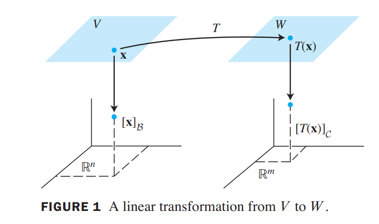
Let $V$ be an $n$-dimensional vector space, let $W$ be an $m$-dimensional vector space, and let $T$ be any linear transformation from $V$ to $W$ . To associate a matrix with $T$, choose (ordered) bases $\beta$ and $\gamma$ for $V$ and $W$ , respectively.

Given any $\vec{x}$ in $V$ , the coordinate vector $\begin{bmatrix}\vec{x}\end{bmatrix}_\beta$ is in $R^n$ and the coordinate vector of its image, $\begin{bmatrix}T(\vec{x})\end{bmatrix}_\gamma$, is in $R^m$, as shown in Figure 1.

The connection between $\begin{bmatrix}\vec{x}\end{bmatrix}_\beta$ and $\begin{bmatrix}T(\vec{x})\end{bmatrix}_\gamma$ is easy to find. Let $\lbrace \vec{b_1}, \cdots, \vec{b_n} \rbrace$ be the basis $\beta$ for $V$ . If $\vec{x} = r_1\vec{b_1} + \cdots + r_n\vec{b_n}$, then
$$
\begin{bmatrix} \vec{x}_\beta\end{bmatrix}=
\begin{bmatrix}r_1 \\ \cdots \\r_n\end{bmatrix}
$$
and
$$
T(\vec{x}) = T(r_1\vec{b_1} + \cdots + r_n\vec{b_n})
= r_1T(\vec{b_1}) + \cdots + r_nT(\vec{b_n})\tag{1}
$$
because $T$ is linear. Now, since the coordinate mapping from $W$ to $R^m$ is linear, equation (1) leads to
$$
\begin{bmatrix} T(\vec{x}) \end{bmatrix}_\gamma = r_1\begin{bmatrix} T(\vec{b_1}) \end{bmatrix}_\gamma\ +
\cdots + r_n\begin{bmatrix} T(\vec{b_n}) \end{bmatrix}_\gamma\tag{2}
$$
Since $C$-coordinate vectors are in $R^m$, the vector equation (2) can be written as a matrix equation, namely,
$$
\begin{bmatrix}
T(\vec{x})
\end{bmatrix}_\gamma =
M\begin{bmatrix}
\vec{x}
\end{bmatrix}_\beta\tag{3}
$$
where

$$
M = \begin{bmatrix}
\begin{bmatrix}
(T(\vec{b_1}))
\end{bmatrix}_\gamma
&
\begin{bmatrix}
(T(\vec{b_2}))
\end{bmatrix}_\gamma
&
\cdots
&
\begin{bmatrix}
(T(\vec{b_n}))
\end{bmatrix}_\gamma
\end{bmatrix}\tag{4}
$$
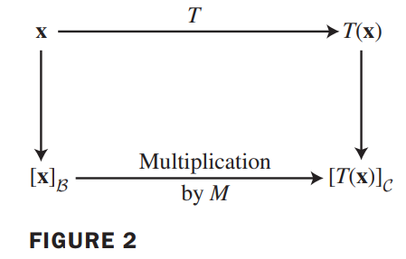
The matrix $M$ is a matrix representation of $T$ , called the matrix for $T$ relative to the bases $\beta$ and $\gamma$. See Figure 2.

💡For Example💡:

Suppose $\beta = \lbrace \vec{b_1}, \vec{b_2}\rbrace$ is a basis for $V$ and $\gamma = \lbrace \vec{c_1}, \vec{c_2}, \vec{c_3}\rbrace$ is a basis for $W$. Let $T: V \rightarrow W$ be a linear transformation with the property that

$$
T(\vec{b_1}) = 3\vec{c_1} - 2\vec{c_2} + 5\vec{c_3}\\
T(\vec{b_2}) = 4\vec{c_1} + 7\vec{c_2} - \vec{c_3}
$$
Find the matrix $M$ for $T$ relative to $\beta$ and $\gamma$.

Solution:

The $\gamma$-coordinate vectors of the images of $\vec{b_1}$ and $\vec{b_2}$ are

$$
\begin{bmatrix}
T(\vec{b_1})
\end{bmatrix}_\gamma =
\begin{bmatrix}
3 \\ -2 \\ 5
\end{bmatrix}\
\begin{bmatrix}
T(\vec{b_2})
\end{bmatrix}_\gamma =
\begin{bmatrix}
4 \\ 7 \\ -1
\end{bmatrix}
$$
Hence,
$$
M =
\begin{bmatrix}
3 & 4\\ -2 & 7\\ 5 & -1
\end{bmatrix}
$$

Linear Transformations on $R^n$

Diagonal Matrix Representation
Suppose $A = PDP^{-1}$, where $D$ is a diagonal $n \times n$ matrix. If $\beta$ is the basis for $R^n$ formed from the columns of $P$ , then $D$ is the $\beta-matrix$ for the transformation $x \mapsto Ax$.

💡For example💡:

Define $T: R^2\mapsto R^2$ by $T(\vec{x}) = A\vec{x}$, where $A = \begin{bmatrix} 7 & 2\\-4 & 1\end{bmatrix}$. Find a basis $\beta$ for $R^2$ with the property that the $\beta-matrix$ for $T$ is a diagonal matrix.

Solution:

$$
A = PDP^{-1}, P = \begin{bmatrix}1 & 1 \\ -1 & -2\end{bmatrix}
, D = \begin{bmatrix}5 & 0 \\ 0 & 3\end{bmatrix}
$$
The columns of $P$ , call them $\vec{b_1}$ and $\vec{b_2}$, are eigenvectors of $A$. Thus, $D$ is the $B-matrix$ for $T$ when $\beta = \lbrace \vec{b_1}, \vec{b_2} \rbrace$. The mappings$\vec{x} \mapsto A\vec{x}$ and $\vec{u} \mapsto D\vec{u}$ describe the same linear transformation, relative to different bases.

Complex EigenValues

$C^n$: a space of $n$-tuples of complex numbers.

💡For Example💡:

If $A = \begin{bmatrix} 0 & -1 \\ 1 & 0 \end{bmatrix}$, then the linear transformation $\vec{x} \mapsto A\vec{x}$ on $R^2$ rotates the plane counterclockwise through a quarter-turn.The action of $A$ is periodic, since after four quarter-turns, a vector is back where it started. Obviously, no nonzero vector is mapped into a multiple of itself, so $A$ has no eigenvectors in $R^2$ and hence no real eigenvalues. In fact, the characteristic equation of $A$ is

$$
\lambda^2 + 1 = 0\rightarrow
\lambda = i, \lambda = -i;
$$
If we permit $A$ to act on $C^2$, then

$$
\begin{bmatrix}
0 & -1\\
1 & 0
\end{bmatrix}
\begin{bmatrix}
1 \\ -i
\end{bmatrix}=
i\begin{bmatrix}
1 \\ -i
\end{bmatrix}
\\
\begin{bmatrix}
0 & -1\\
1 & 0
\end{bmatrix}
\begin{bmatrix}
1 \\ i
\end{bmatrix}=
-i\begin{bmatrix}
1 \\ i
\end{bmatrix}
$$
Thus, $i,-i$ are eigenvalues, with $\begin{bmatrix}1 \\ -i\end{bmatrix}$ and $\begin{bmatrix}1 \\ i\end{bmatrix}$ as corresponding eigenvectors.

💡For Example💡:

Let $A = \begin{bmatrix} 0.5 & -0.6 \\ 0.75 & 1.1 \end{bmatrix}$. Find the eigenvalues of $A$, and find a basis for each eigenspace.

Solution:

$$
0 = det
\begin{bmatrix}
0.5-\lambda & -0.6 \\ 0.75 & 1.1-\lambda
\end{bmatrix}
=\lambda^2 - 1.6\lambda + 1\\
\Rightarrow
\lambda = 0.8 \pm 0.6i
$$
for $\lambda = 0.8 - 0.6i$, construct

$$
A - (0.8-0.6i)I =
\begin{bmatrix}
-0.3 + 0.6i & -0.6\\
0.75 & 0.3 + 0.6i
\end{bmatrix}\tag{2}
$$
The second equation in (2) leads to

$$
0.75x_1 = (-0.3-0.6i)x_2\\
x_1 = (-0.4-0.8i)x_2
$$
Choose $x_2 = 5$ to eliminate the decimals, and obtain $x_1 = -2 - 4i$.

$$
\vec{v_1} = \begin{bmatrix}
-2-4i\\
5
\end{bmatrix}
$$
Analogous calculations for $\lambda = 0.8 + 0.6i$ produce the eigenvector

$$
\vec{v_2} = \begin{bmatrix}
-2 + 4i\\
5
\end{bmatrix}
$$
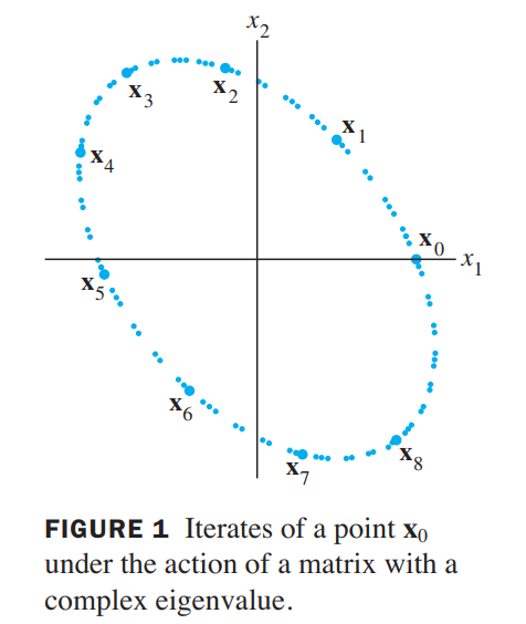
the matrix $A$ determines a transformation $\vec{x} \mapsto A\vec{x}$ that is essentially a rotation. See Figure1.

Real and Imaginary Parts of Vectors

💡For Example💡:

If $\vec{x} = \begin{bmatrix}3-i\\i\\2+5i\end{bmatrix}$ = $\begin{bmatrix}3\\0\\2\end{bmatrix}$ + i$\begin{bmatrix}-1\\1\\5\end{bmatrix}$, then

$$
Re(Real)\vec{x} = \begin{bmatrix}3 \\ 0 \\ 2\end{bmatrix}\\
Im(Imaginary)\vec{x} = \begin{bmatrix}-1 \\ 1 \\ 5\end{bmatrix}, and \overline{\vec{x}} = \begin{bmatrix}3\\0\\2\end{bmatrix} - i\begin{bmatrix}-1\\1\\5\end{bmatrix}
$$

Eigenvalues and Eigenvectors of a Real Matrix That Acts on $C^n$

💡For Example💡:

If $C = \begin{bmatrix}a & -b \\ b & a\end{bmatrix}$, where $a$ and $b$ are real and not both zero, then the eigenvalues of $C$ are $\lambda = a \pm bi$. Also, if $r = |\lambda| = \sqrt{a^2 + b^2}$, then

$$
C = r
\begin{bmatrix}
a/r & -b/r\\
b/r & a/r
\end{bmatrix} =
\begin{bmatrix}
r & 0\\
0 & r
\end{bmatrix}
\begin{bmatrix}
\cos\psi & -\sin\psi\\
\sin\psi & \cos\psi
\end{bmatrix}
$$

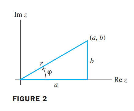
where $\psi$ is the angle between the positive $x-axis$ and the ray from $(0,0)$ through $(a,b)$. The angle $\psi$ is called the argument of $\lambda = a + bi$.

Thus the transformation $\vec{x}\mapsto C\vec{x}$ may be viewed as the composition of a rotation through the angle $\psi$ and a scaling by $|\lambda|$ (see Figure 3).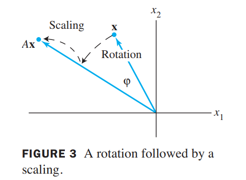

Let $A$ be a real $2 \times 2$ matrix with a complex eigenvalue $\lambda = a - bi, b \neq 0$ and an associated eigenvector $\vec{v}$ in $C^2$. Then

$$
A = PCP^{-1}, where \space P = \begin{bmatrix} Re\vec{v} & Im\vec{v}\end{bmatrix}
and \space C = \begin{bmatrix}a & -b\\ b & a\end{bmatrix}
$$
💡For Example💡:

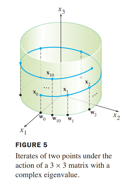
The matrix $A = \begin{bmatrix}0.8 & -0.6 & 0\\0.6 & 0.8 & 0\\ 0 & 0 & 1.07\end{bmatrix}$ has eigenvalues $0.8\pm 0.6i$ and $1.07$. Any vector $\vec{w_0}$ in the $x_1x_2-plane$ (with third coordinate 0) is rotated by $A$ into another point in the plane. Any vector $\vec{x_0}$ not in the plane has its $x_3-coordinate$ multiplied by $1.07$. The iterates of the points $\vec{w_0} = (2,0,0)$ and $\vec{x_0} = (2,0,1)$ under multiplication by $A$ are shown in Figure 5.

👉More about Complex EigenValues and Quaternions >>

Discrete Dynamical Systems(Omitted)

Applications to Differential Equations 微分方程

$$
\vec{x(t)’} = A\vec{x(t)}
$$

where,
$$
\vec{x(t)} =
\begin{bmatrix}
x_1(t)\\
\cdots\\
x_n(t)
\end{bmatrix},
\vec{x’(t)} =
\begin{bmatrix}
x_1’(t)\\
\cdots\\
x_n’(t)
\end{bmatrix},
A =
\begin{bmatrix}
a_{11} & \cdots & a_{1n}\\
\cdots& & \cdots\\
a_{n1} & \cdots & a_{nn}
\end{bmatrix}
$$
$x_1, x_2, \cdots, x_n$ are differentiable functions of $t$.

👉First-order Differential Equation >>

💡For example💡 :

$$
\begin{bmatrix}
x_1’(t)\\
x_2’(t)
\end{bmatrix}
=
\begin{bmatrix}
3 & 0\\
0 & -5
\end{bmatrix}
\begin{bmatrix}
x_1(t)\\
x_2(t)
\end{bmatrix}
\tag{2}
$$

$$
\begin{cases}
x_1’(t) = 3x_1(t)\\
x_2’(t) = -5x_2(t)
\end{cases}
\tag{3}
$$

The system (2) is said to be decoupled because each derivative of a function depends only on the function itself, not on some combination or “coupling” of both $x_1(t)$ and $x_2(t)$. From calculus, the solutions of (3) are $x_1(t) = c_1e^{3t}$ and $x_2(t) = c_2e^{-5t}$, for any constants $c_1$ and $c_2$. Each solution of equation (2) can be written in the form

$$
\begin{bmatrix}
x_1(t)\\
x_2(t)
\end{bmatrix}
=
\begin{bmatrix}
c_1e^{3t}\\
c_2e^{-5t}
\end{bmatrix}
=
c_1\begin{bmatrix}
1 \\
0
\end{bmatrix}
e^{3t}
+
c_2\begin{bmatrix}
0 \\
1
\end{bmatrix}
e^{-5t}
$$
This example suggests that for the general equation $\vec{x}’ = A\vec{x}$, a solution might be a linear combination of functions of the form

$$
\vec{x}(t) = \vec{v} e^{\lambda t}
\tag{4}
$$

Thus,
$$
\begin{cases}
\vec{x’}(t) = \lambda \vec{v} e^{\lambda t}\\
A\vec{x}(t) = A\vec{v} e^{\lambda t}
\end{cases}
\Rightarrow
A\vec{v} = \lambda\vec{v}
$$

that means, $\lambda$ is an eigenvalue of $A$ and $\vec{v}$ is a corresponding eigenvector.

Eigenfunctions provide the key to solving systems of differential equations.

💡For example💡:

Suppose a particle is moving in a planar force field and its position vector $\vec{x}$ satisfies $\vec{x’} = A\vec{x}$ and $\vec{x}(0) = \vec{x_0}$, where

$$
A =
\begin{bmatrix}
4 & -5\\
-2 & 1
\end{bmatrix}
,
\vec{x_0} =
\begin{bmatrix}
2.9\\
2.6
\end{bmatrix}
$$
Solve this initial value problem for $t \geq 0$ and sketch the trajectory of the particle.

Solution:

the eigenvalues of A is $\lambda_1 = 6, \lambda_2 = -1$, with corresponding eigenvectors $\vec{v_1} = (-5,2), \vec{v_2} = (1,1)$. So the function is

$$
\begin{aligned}
\vec{x}(t) &= c_1\vec{v_1}e^{\lambda_1t} + c_2\vec{v_2}e^{\lambda_2t}
\\
&= c_1\begin{bmatrix}-5 \\ 2\end{bmatrix} e^{6t} + c_2\begin{bmatrix}1 \\ 1\end{bmatrix} e^{-t}
\end{aligned}
$$
is the solution of $\vec{x’} = A\vec{x}$.

$$
\vec{x}(0) = \vec{x_0} \longrightarrow
c_1\begin{bmatrix}-5 \\ 2\end{bmatrix} + c_2\begin{bmatrix}1 \\ 1\end{bmatrix} =
\begin{bmatrix}
2.9\\
2.6
\end{bmatrix}
$$
Thus,
$$
\vec{x}(t) = \frac{-3}{70}\begin{bmatrix}-5 \\ 2\end{bmatrix} e^{6t} + \frac{188}{70}\begin{bmatrix}1 \\ 1\end{bmatrix} e^{-t}
$$

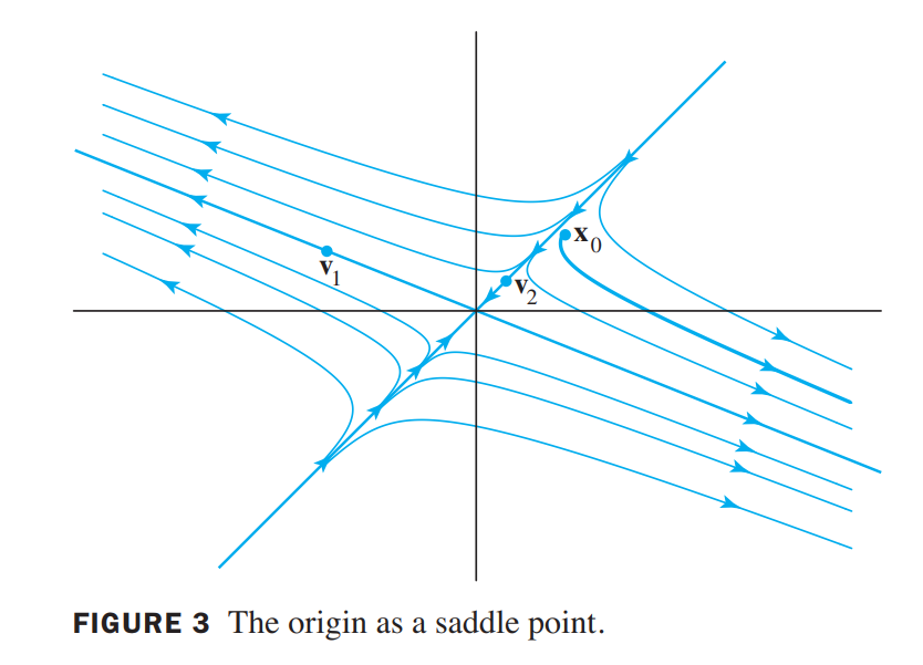
See Figure3, the origin is called a saddle point of the dynamical system because some trajectories approach the origin at first and then change direction and move away from the origin. A saddle point arises whenever the matrix $A$ has both positive and negative eigenvalues. The direction of greatest repulsion is the line through $\vec{v_1}$ and $\vec{0}$, corresponding to the positive eigenvalue. The direction of greatest attraction is the line through $\vec{v_2}$ and $\vec{0}$, corresponding to the negative eigenvalue.

Iterative Estimates for Eigenvalues 迭代估计特征值(Numerical Analysis)

The Power Method

The power method applies to an $n \times n$ matrix $A$ with a strictly dominant eigenvalue $\lambda_1$, which means that $\lambda_1$ must be larger in absolute value than all the other eigenvalues.

The Power Method For Estimating A Strictly Dominant EigenValue

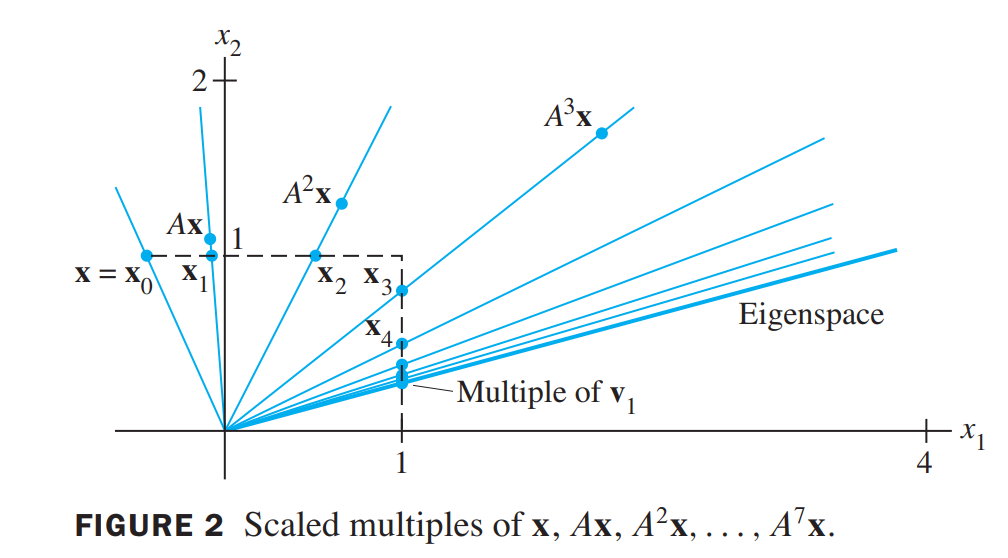
1. Select an initial vector $\vec{x_0}$ whose largest entry is 1.
2. For k = 0, 1 …
   a. Compute $A\vec{x_k}$.
   b. Let $\mu_k$ be an entry in $A\vec{x_k}$ whose absolute value is as large as possible.
   c. Compute $\vec{x_{k+1}} = (\frac{1}{\mu_k})A\vec{x_k}$.
3. For almost all choices of $\vec{x_0}$, the sequence $\lbrace \mu_k \rbrace$ approaches the dominant eigenvalue, and the sequence $\lbrace \vec{x_k} \rbrace$ approaches a corresponding eigenvector.

The Inverse Power Method

This method provides an approximation for any eigenvalue, provided a good initial estimate $\alpha$ of the eigenvalue $\lambda$ is known.

The Inverse Power Method For Estimating An EigenValue $\lambda$ of $A$

1. Select an initial estimate $\alpha$ sufficiently close to $\lambda$.
2. Select an initial vector $\vec{x_0}$ whose largest entry is 1.
3. For k = 0, 1 …
   a. Solve $(A - \alpha I)\vec{y_k} = \vec{x_k}$ for $\vec{y_k}$.
   b. Let $\mu_k$ be an entry in $\vec{y_k}$ whose absolute value is as large as possible.
   c. Compute $v_{k} = \alpha + (1/\mu_k)$.
   d. Compute $\vec{x_{k+1}} = (1/\mu_k)\vec{y_k}$
4. For almost all choices of $\vec{x_0}$, the sequence $\lbrace v_k \rbrace$ approaches the eigenvalue $\lambda$ of $A$, and the sequence $\lbrace \vec{x_k} \rbrace$ approaches a corresponding eigenvector.

👉More about Calculate EigenValues by Numerical Analysis >>