Keywords: Affine Combinations, Barycentric Coordinates,Bézier Curves
This is the Chapter8 ReadingNotes from book Linear Algebra and its Application.
Affine Combinations
An affine combination of vectors is a special kind of linear combination.Given vectors (or “points”) $v_1, v_2, \cdots, v_p$ in $R^n$ and scalars $c_1, \cdots, c_p$, an affine combination of $v_1, v_2, \cdots, v_p$ is a linear combination
$$
c_1v_1 + \cdots + c_pv_p,\\ c_1 + \cdots + c_p = 1
$$
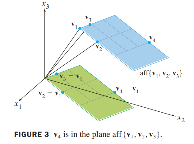
A point $y$ in $R^n$ is an affine combination of $v_1, \cdots v_p$ in $R^n$ if and only if $(y - v_1)$ is a linear combination of the translated points $v_2 - v_1, \cdots, v_p - v_1$.
Affine Independence
An indexed set of points $v_1, … v_p$ in $R^n$ is affinely dependent if there exist real numbers $c_1, .. c_p$, not all zero, such that
$$
c_1 + \cdots + c_p = 0 \space and \space c_1v_1 + \cdots + c_pv_p = 0
$$
Otherwise, the set is affinely independent.
Given an indexed set $S = \lbrace v_1, \cdots, v_p \rbrace$ in $R^n$, with $p \geq 2$,the following statements are logically equivalent. That is, either they are all true statements or they are all false.
a. $S$ is affinely dependent.
b. One of the points in $S$ is an affine combination of the other points in $S$.
c. The set $\lbrace v_2 - v_1, \cdots v_p - v_1\rbrace$ in $R^n$ is linearly dependent.
d. The set $\widetilde{v_1}, \cdots, \widetilde{v_p}$ of homogeneous forms in $R^{n+1}$ is linearly dependent.
💡For example💡:
let $\vec{v_1} = \begin{bmatrix} 1 \\ 3 \\ 7\end{bmatrix}, \vec{v_2} = \begin{bmatrix} 2 \\ 7 \\ 6.5\end{bmatrix}, \vec{v_3} = \begin{bmatrix} 0 \\ 4 \\ 7\end{bmatrix}, \vec{v_4} = \begin{bmatrix} 0 \\ 14 \\ 6\end{bmatrix}$, and $S = \lbrace \vec{v_1}, \vec{v_2}, \vec{v_3}, \vec{v_4} \rbrace$. Determine whether $S$ is affinely independent.
Solution:
$$
\vec{v_2} -\vec{v_1} = \begin{bmatrix} 1 \\ 4 \\ -0.5\end{bmatrix},
\vec{v_3} -\vec{v_1} = \begin{bmatrix} -1 \\ 1 \\ 0\end{bmatrix},
\vec{v_4} -\vec{v_1} = \begin{bmatrix} -1 \\ 11 \\ -1\end{bmatrix}
\Rightarrow
\begin{bmatrix}
1 & -1 & -1\\
4 & 1 & 11\\
-0.5 & 0 & -1
\end{bmatrix}
\sim
\begin{bmatrix}
1 & -1 & -1\\
0 & 5 & 15\\
0 & 0 & 0
\end{bmatrix}
$$
the columns are linearly dependent because not every column is a pivot column, so $v_2 - v_1, v_3 - v_1, v_4 - v_1$ are linearly dependent.
Thus, $v_1, v_2, v_3, v_4$ is affinely dependent.
$$
\vec{v_4} - \vec{v_1} = 2(\vec{v_2} - \vec{v_1}) + 3(\vec{v_3} - \vec{v_1})\\
\vec{v_4} = -4\vec{v_1} + 2\vec{v_2} + 3\vec{v_3}
$$
Barycentric Coordinates
let $S = \lbrace \vec{v_1},\cdots, \vec{v_k}\rbrace$ be an affinely independent set in $R^n$. Then each $\vec{p}$ in aff S has a unique representation as an affine combination of $\vec{v_1},\cdots,\vec{v_k}$. That is, for each $\vec{p}$ there exists a unique set of scalars $c_1, \cdots, c_k$ such that
$$
\vec{p} = c_1\vec{v_1} + \cdots + c_k\vec{v_k}, and \space c_1 + \cdots + c_k = 1 \tag{7}
$$
the coefficients $c_1 \cdots c_k$ in the unique representation (7) of $\vec{p}$ are called the barycentric (or, sometimes, affine) coordinates of $\vec{p}$
Observe that (7) is equivalent to the single equation
$$
\begin{bmatrix}
\vec{p}\\1
\end{bmatrix} = c_1\begin{bmatrix} \vec{v_1}\\1 \end{bmatrix} + \cdots + c_k\begin{bmatrix} \vec{v_k }\\1
\end{bmatrix}
\tag{8}
$$
involving the homogeneous forms of the points. Row reduction of the augmented matrix $\begin{bmatrix} \widetilde{\vec{v_1}} & \cdots \widetilde{\vec{v_k}} & \widetilde{\vec{p}}\end{bmatrix}$ for (8) produces the barycentric coordinates of $\vec{p}$.
💡For Example💡:
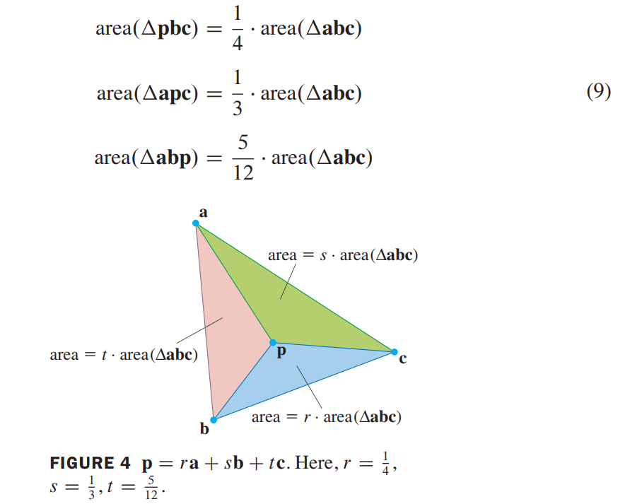
Let $\vec{a} = \begin{bmatrix} 1 \\ 7\end{bmatrix}, \vec{b} = \begin{bmatrix} 3 \\ 0\end{bmatrix}, \vec{c} = \begin{bmatrix} 9 \\ 3\end{bmatrix}, and \space \vec{p} = \begin{bmatrix} 5 \\ 3\end{bmatrix}$ Find the barycentric coordinates of $\vec{p}$ determined by the affinely independent set $\lbrace \vec{a}, \vec{b}, \vec{c}\rbrace$.
👉Solution:
$$
\begin{bmatrix}
\widetilde{\vec{a}} & \widetilde{\vec{b}} & \widetilde{\vec{c}} & \widetilde{\vec{p}}
\end{bmatrix}
=
\begin{bmatrix}
1 & 3 & 9 & 5\\
7 & 0 & 3 & 3\\
1 & 1 & 1 & 1
\end{bmatrix}
\sim
\begin{bmatrix}
1 & 0 & 0 & \frac{1}{4}\\
7 & 0 & 3 & \frac{1}{3}\\
1 & 1 & 1 & \frac{5}{12}
\end{bmatrix}
$$
so, $\vec{p} = \frac{1}{4}\vec{a} + \frac{1}{3}\vec{b} + \frac{5}{12}\vec{c}$
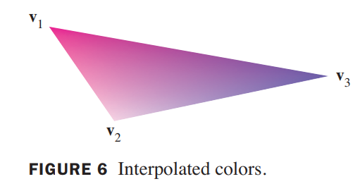
Barycentric Coordinates in Computer Graphics
Barycentric coordinates provide the tool for smoothly interpolating the vertex information over the interior of a triangle.
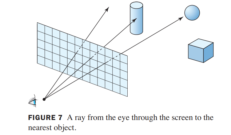
The color and other information displayed in the pixel on the screen should come from the object that the ray first intersects. See Figure 7. When the objects in the graphics scene are approximated by wire frames with triangular patches, the hidden surface problem can be solved using barycentric coordinates.
💡For example💡:
Let
$$
\vec{v_1} =
\begin{bmatrix}
1\\
1\\
-6
\end{bmatrix},
\vec{v_2} =
\begin{bmatrix}
8\\
1\\
-4
\end{bmatrix},
\vec{v_3} =
\begin{bmatrix}
5\\
11\\
-2
\end{bmatrix},
\vec{a} =
\begin{bmatrix}
0\\
0\\
10
\end{bmatrix},
\vec{b} =
\begin{bmatrix}
0.7\\
0.4\\
-3
\end{bmatrix}
$$
and $x(t) = a + tb$ for $t \geq 0$. Find the point where the ray $x(t)$ intersects the plane that contains the triangle with vertices $v_1, v_2, and v_3$. Is this point inside the triangle?
Solution:
The plane is $aff \lbrace \vec{v_1}, \vec{v_2}, \vec{v_3} \rbrace$. The ray $x(t)$ intersects the plane when $c_2, c_3$, and $t$ satisfy
$$
(1-c_2-c_3)\vec{v_1} + c_2\vec{v_2} + c_3\vec{v_3} = \vec{a} + t\vec{b} \mapsto\\
\begin{bmatrix}
\vec{v_2} - \vec{v_1} & \vec{v_3} - \vec{v_1} & -\vec{b}
\end{bmatrix}
\begin{bmatrix}
c_2 \\ c_3 \\ t
\end{bmatrix}
=
\vec{a} - \vec{v_1}
$$
thus, get the solution and the intersection point is
$$
\vec{x(5)} = \vec{a} + 5\vec{b} = \begin{bmatrix} 3.5 \\ 2.0 \\ -5.0\end{bmatrix}
$$
The intersection point is inside the triangle because the barycentric weights for $\vec{x(5)}$ are all positive.
Convex Combinations(凸包)
A convex combination of points $\vec{v_1}, \vec{v_2},\cdots, \vec{v_k}$ in $R^n$ is a linear combination of the form
$$
c_1\vec{v_1} + c_2\vec{v_2} + \cdots + c_k\vec{v_k}
$$
such that $c_1 + c_2 + \cdots + c_k = 1$ and $c_i \geq 0$ for all $i$. The set of all convex combinations of points in a set $S$ is called the convex hull of $S$, denoted by $conv S$.
the point in $cov \lbrace \vec{v_1}, \vec{v_2} \rbrace$ may be written as
$$
\vec{y} = (1-t)\vec{v_1} + t\vec{v_2} , 0 \leq t \leq 1
$$
which is a line segment between $\vec{v_1}$ and $\vec{v_2}$, hereafter denoted by $\overline{\vec{v_1}\vec{v_2}}$
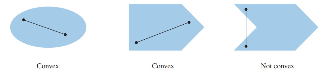
A set $S$ is convex if for each $\vec{p}, \vec{q} \in S$, the line segment $\overline{\vec{p}\vec{q}}$ is contained in $S$.
Intuitively, a set $S$ is convex if every two points in the set can “see” each other without the line of sight leaving the set. Figure 1 illustrates this idea.
consider a set $S$ that lies inside some large rectangle in $R^2$, and imagine stretching a rubber band around the outside of $S$. As the rubber band contracts around $S$, it outlines the boundary of the convex hull of $S$. Or to use another analogy, the convex hull of $S$ fills in all the holes in the inside of $S$ and fills out all the dents in the boundary of $S$.
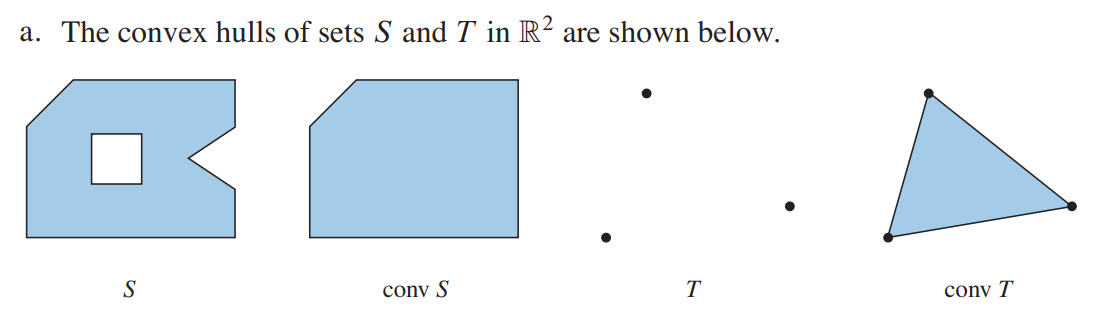
A set $S$ is convex if and only if every convex combination of points of $S$ lies in $S$. That is, $S$ is convex if and only if $S$ = $conv S$.
👉More about ConvexHull Algorithms>>
Hyperplanes(超平面)
The key to working with hyperplanes is to use simple implicit descriptions, rather than the explicit or parametric representations of lines and planes used in the earlier work with affine sets.
An implicit equation of a line in $R^2$ has the form $ax + by = d$. An implicit equation of a plane in $R^3$ has the form $ax + by + cz = d$. Both equations describe the line or plane as the set of all points at which a linear expression (also called a linear functional(线性泛函)) has a fixed value, d.
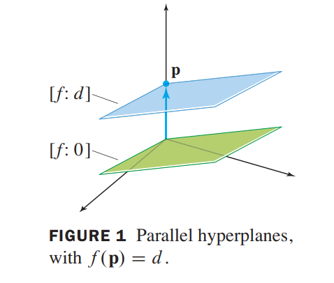
A linear functional on $R^n$ is a linear transformation $f$ from $R^n$ into $R$. For each
scalar $d$ in $R$, the symbol $[f:d]$ denotes the set of all $\vec{x}$ in $R^n$ at which the value
of $f$ is $d$. That is,
$$
[f:d] \space is \space the \space set \lbrace \vec{x} \in R^n : f(\vec{x}) = d\rbrace
$$
line: $x - 4y = 13$, is a hyperplane in $R^2$, it is the set of points at which the linear functional $f(x,y) = x - 4y$ has the value 13, the line is the set $[f:13]$
If $f$ is a linear functional on $R^n$, then the standard matrix of this linear transformation $f$ is a $1 \times n$ matrix $A$, say $A = \begin{bmatrix}a_1 & a_2 & \cdots & a_n \end{bmatrix}$. So
$$
[f:0] \Leftrightarrow \lbrace \vec{x} \in R^n: A\vec{x} = \vec{0}\rbrace \Leftrightarrow NullA
$$
We know the relation between $A\vec{x} = \vec{0}$ and $A\vec{x} = \vec{b}$, thus
$$
[f:d] = [f:0] + \vec{p}, \vec{p} \in [f:d]
$$
$$
[f:0] = \lbrace \vec{x} \in R^n: \vec{n} \cdot \vec{x} = 0\rbrace
$$
$\vec{n}$ is called a normal vector(法向量) to $[f:0]$, sometimes it’s also called gradient(梯度).
💡For example💡:
In $R^2$, give an explicit description of the line $x-4y = 13$ in parametric vector form.
Solution:
$$
\begin{aligned}
\vec{x} &= \begin{bmatrix}x \\ y\end{bmatrix}= \begin{bmatrix}13 + 4y \\ y\end{bmatrix}\\
&= \begin{bmatrix} 13 \\ 0\end{bmatrix} + y \begin{bmatrix} 4 \\ 1\end{bmatrix} = \vec{p} + y\vec{q}
\end{aligned}
$$
💡For example💡:
Let $\vec{v_1} = \begin{bmatrix} 1 \\ 1 \\ 1\end{bmatrix}, \vec{v_2} = \begin{bmatrix} 2 \\ -1 \\ 4\end{bmatrix}, \vec{v_3} = \begin{bmatrix} 3 \\ 1 \\ 2\end{bmatrix}$. Find an implicit description $[f : d]$ of the plane $H_1$ that passes through $\vec{v_1}, \vec{v_2}, \vec{v_3}$.
Solution:
$H_1$ is parallel to a plane $H_0$ through the origin that contains the translated points
$$
\vec{v_2} - \vec{v_1} =
\begin{bmatrix}
1 \\ -2 \\ 3
\end{bmatrix},
\vec{v_3} - \vec{v_1} =
\begin{bmatrix}
2 \\ 0 \\ 1
\end{bmatrix}
$$
Since these two points are linearly independent, $H_0 = Span \lbrace \vec{v_2} - \vec{v_1}, \vec{v_3} - \vec{v_1} \rbrace$. Let $\vec{n} = \begin{bmatrix} a \\ b \\ c\end{bmatrix}$ be the normal to $H_0$.
$$
\begin{bmatrix} 1 & -2 & 3\end{bmatrix} \begin{bmatrix} a \\ b \\ c\end{bmatrix} = 0,
\begin{bmatrix} 2 & 0 & 1\end{bmatrix} \begin{bmatrix} a \\ b \\ c\end{bmatrix} = 0
\Longrightarrow \\
\begin{bmatrix} 1 & -2 & 3 & 0\\ 2 & 0 & 1 & 0\end{bmatrix}
\Longrightarrow \\
\vec{n} = \begin{bmatrix} -2 \\ 5 \\ 4\end{bmatrix}
$$
or
$$
\begin{aligned}
\vec{n} &= (\vec{v_2} - \vec{v_1}) \times (\vec{v_3} - \vec{v_1})\\
&= \left|
\begin{array}{cccc}
1 & 2 & i \\
-2 & 0 & j \\
3 & 1 & k
\end{array}
\right|\\
&= -2i + 5j + 4k
\end{aligned}
$$
Thus,
$$
f(x) = -2x_1 + 5x_2 + 4x_3 \\
d = f(\vec{v_1}) = 7
\Longrightarrow
H_1 : [f: d]
$$
A subset $H$ of $R^n$ is a hyperplane if and only if $H = [f:d]$ for some nonzero linear functional $f$ and some scalar $d$ in $R$. Thus, if $H$ is a hyperplane, there exist a nonzero vector $\vec{n}$ and a real number $d$ such that $H = \lbrace \vec{x} : \vec{n} \cdot \vec{x} = d\rbrace$.
Topology in $R^n$
For any point $p$ in $R^n$ and any real $\delta > 0$, the open ball $B(p,\delta)$ with center $p$ and radius $\delta$ is given by
$$
B(p,\delta) = \lbrace x : ||x - p|| < \delta\rbrace
$$
Given a set in $R^n$,
A set is open if it contains none of its boundary points.
A set is closed if it contains all of its boundary points.
A set $S$ is bounded if there exists a $\delta > 0$ such that $S \subset B(0, \delta)$.
A set in $R^n$ is compact if it is closed and bounded.
Polytopes(多面体)
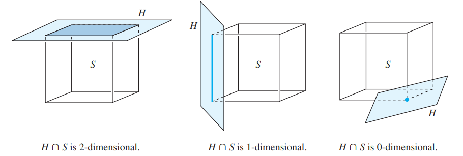
Let $S$ be a compact convex subset of $R^n$. A nonempty subset $F$ of $S$ is called a (proper) face of $S$ if $F \neq S$ and there exists a hyperplane $H = [f:d]$ such that $F = S \cap H$ and either $f(S) \leq d$ or $f(S) > \geq d$. The hyperplane $H$ is called a supporting hyperplane to $S$. If the dimension of $F$ is $k$, then $F$ is called a $k-face$ of $S$.
If $P$ is a polytope of dimension $k$, then $P$ is called a $k-polytope$. A $0-face$ of $P$ is called a vertex (plural: vertices), a $1-face$ is an edge, and a $(k-1)-dimensional$ face is a facet of $S$.
Simplex
HyperCube(超立方体)
Curves and Surfaces
Bézier Curves
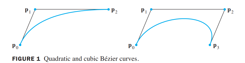
quadratic and cubic Bézier curves:
$$
\begin{aligned}
&\vec{w(t)} = (1-t^2)\vec{p_0} + 2t(1-t)\vec{p_1} + t^2\vec{p_2}\\
&\vec{x(t)} = (1-t^3)\vec{p_0} + 3t(1-t)^2\vec{p_1} + 3t^2(1-t)\vec{p_2} + t^3\vec{p_3}\\
\end{aligned}
$$
Bézier curves are useful in computer graphics because their essential properties are preserved under the action of linear transformations and translations.
$$
\begin{aligned}
A\vec{x(t)} &= A[(1-t^3)\vec{p_0} + 3t(1-t)^2\vec{p_1} + 3t^2(1-t)\vec{p_2} + t^3\vec{p_3}]\\
&= (1-t^3)A\vec{p_0} + 3t(1-t)^2A\vec{p_1} + 3t^2(1-t)A\vec{p_2} + t^3A\vec{p_3}
\end{aligned}
$$
the new control points are $A\vec{p_0}, \cdots, A\vec{p_3}$.
Connecting Two Bézier Curves
The combined curve is said to have $G^0$ geometric continuity (at $p_2$) because the two segments join at $p_2$.
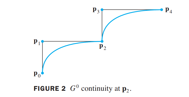
To avoid a sharp bend, it usually suffices to adjust the curves to have what is called $G^1$ geometric continuity, where both tangent vectors at $p_2$ point in the same direction.
When the tangent vectors are actually equal at $p_2$, the tangent vector is continuous at $p_2$, and the combined curve is said to have $C^1$ continuity, or $C^1$ parametric continuity.
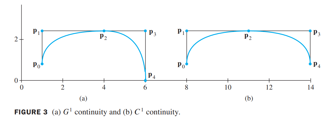
Figure 4 shows $C^1$ continuity for two cubic Bézier curves. Notice how the point joining the two segments lies in the middle of the line segment between the adjacent control points.
Two curves have $C^2$ (parametric) continuity when they have $C^1$ continuity and the second derivatives are equal. Another class of cubic curves, called B-splines, always have $C^2$ continuity because each pair of curves share three control points rather than one.
Matrix Equations for Bézier Curves
Since a Bézier curve is a linear combination of control points using polynomials as weights, the formula for $\vec{x(t)}$ may be written as
$$
\begin{aligned}
\vec{x(t)} &= \begin{bmatrix}\vec{p_0} & \vec{p_1} & \vec{p_2} & \vec{p_3}\end{bmatrix}\begin{bmatrix}(1-t)^3 \\ 3t(1-t)^2 \\ 3t^2(1-t) \\ t^3\end{bmatrix}
\\
&=\underbrace{\begin{bmatrix}\vec{p_0} & \vec{p_1} & \vec{p_2} & \vec{p_3}\end{bmatrix}}_{Geometry-matrix: G}
\begin{bmatrix}1 & -3 & 3 & -1\\0 & 3 & -6 & 3\\0 & 0 & 3 & -3\\0 & 0 & 0 & 1\end{bmatrix}
\begin{bmatrix}1 \\ t \\ t^2 \\ t^3\end{bmatrix}\\
\end{aligned}
$$
$$
\Longrightarrow
\vec{x(t)} = GM_B\vec{u(t)},M_B : Bezier-basis-matrix
\tag{4}
$$
A Hermite cubic curve arises when the matrix $M_B$ is replaced by a Hermite basis matrix.
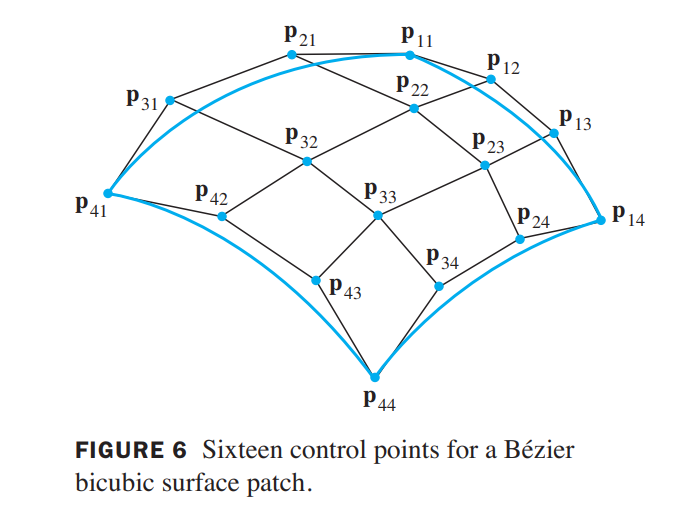
Bézier Surfaces
The Bézier curve in equation (4) can also be “factored” in another way, to be used in the discussion of Bézier surfaces.
$$
\begin{aligned}
\vec{x(s)} &= \vec{u(s)}^TM_B^T\begin{bmatrix}\vec{p_0} \\ \vec{p_1} \\ \vec{p_2} \\ \vec{p_3}\end{bmatrix}\\
&=\begin{bmatrix}1 & s & s^2 & s^3\end{bmatrix}
\begin{bmatrix}1 & 0 & 0 & 0\\-3 & 3 & 0 & 0\\3 & -6 & 3 & 0\\-1 & 3 & -3 & 1\end{bmatrix}
\begin{bmatrix}\vec{p_0} \\ \vec{p_1} \\ \vec{p_2} \\ \vec{p_3}\end{bmatrix}\\
&=\begin{bmatrix} (1-s)^3 & 3s(1-s)^2 & 3s^2(1-s) & s^3\end{bmatrix}
\underbrace{\begin{bmatrix}\vec{p_0} \\ \vec{p_1} \\ \vec{p_2} \\ \vec{p_3}\end{bmatrix}}_{Geometry-vector}
\end{aligned}
$$
Approximations to Curves and Surfaces
The basic idea for approximating a Bézier curve or surface is to divide the curve or surface into smaller pieces, with more and more control points.
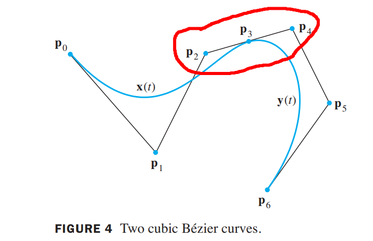
Recursive Subdivision of Bézier Curves and Surfaces
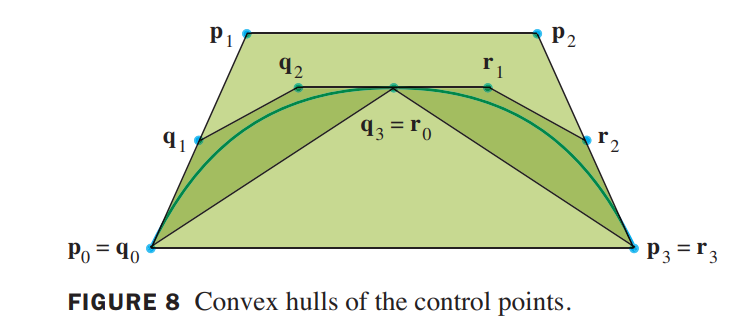
$$
x(t) = (1-3t+3t^2-t^3)p_0 + (3t-6t^2+3t^3)p_1 + (3t^2-3t^3)p_2 + t^3p_3, 0 \leq t \leq 1
$$
Thus, the new control points $q_3$ and $r_0$ are given by
$$
q_3 = r_0 = x(0.5) = \frac{1}{8}(p_0 + 3p_1 + 3p_2 + p_3)
$$
the tangent vector to a parameterized curve $x(t)$ is the derivative $x(t)’$.
$$
x(t)’ = (-3 + 6t -3t^2)p_0 + (3 - 12t + 9t^2)p_1 + (6t-9t^2)p_2 + 3t^2p_3, 0 \leq t \leq 1
$$
In particular,
$$
x’(0) = 3(p_1 - p_0)\\
x’(1) = 3(p_3 - p_2)\\
x’(0.5) = \frac{3}{4}(-p_0 - p_1 + p_2 + p_3)
$$
Let $y(t)$ be the Bézier curve determined by $q_0, \cdots, q_3$, and let $z(t)$ be the Bézier curve determined by $r_0, \cdots, r_3$.
Since $y(t)$ traverses the same path as $x(t)$ but only gets to $x(0.5)$ as $t$ goes from $0$ to $1$,
$$
y(t) = x(0.5t), 0 \leq t \leq 1
$$
Similarly
$$
z(t) = x(0.5 + 0.5t), 0 \leq t \leq 1
$$
By chain rule:
$$
y’(t) = 0.5x’(0.5t),\\
z’(t) = 0.5x’(0.5 + 0.5t)
$$
the control points for $y(t)$ satisfy
$$
3(q_1-q_0) = y’(0) = 0.5x’(0) = \frac{3}{2}(p_1-p_0)\\
3(q_3-q_2) = y’(1) = 0.5x’(0.5) = \frac{3}{8}(-p_0-p_1+p_2+p_3)
$$
Once the subdivision completely stops, the endpoints of each curve are joined by line segments, and the scene is ready for the next step in the final image preparation.

