Keywords: Symmetric Matrix, Quadratic Forms, Constrained Optimization, Singular Value Decomposition, ImageProcessing, Statistics, PCA
This is the Chapter7 ReadingNotes from book Linear Algebra and its Application.
Diagonalization of Symmetric Matrices(对称矩阵的对角化)
If $A$ is symmetric, then any two eigenvectors from different eigenspaces are orthogonal.
An $n \times n$ matrix $A$ is orthogonally diagonalizable if and only if $A$ is a symmetric matrix.
💡For Example💡:
Orthogonally diagonalize the matrix $A = \begin{bmatrix}3 & -2 & 4\\-2 & 6 & 2\\4 & 2 & 3\end{bmatrix}$, whose characteristic equation is
$$
0 = -\lambda^3 + 12\lambda^2 -21\lambda - 98 = -(\lambda - 7)^2(\lambda + 2)
$$
Solution:
$$
\lambda = 7, \vec{v_1} = \begin{bmatrix}1 \\ 0 \\ 1\end{bmatrix},
\vec{v_2} = \begin{bmatrix}-1/2 \\ 1 \\ 0\end{bmatrix};\\
\lambda = -2,\vec{v_3} = \begin{bmatrix}-1 \\ -1/2 \\ 1\end{bmatrix}
$$
Although $\vec{v_1}$ and $\vec{v_2}$ are linearly independent, they are not orthogonal. the component of $\vec{v_2}$ orthogonal to $\vec{v_1}$ is
$$
\vec{z_2} = \vec{v_2} - \frac{\vec{v_2} \cdot \vec{v_1}}{\vec{v_1} \cdot \vec{v_1}}\vec{v_1}
= \begin{bmatrix}
-1/4 \\ 1 \\ 1/4
\end{bmatrix}
$$
Then $\lbrace \vec{v_1}, \vec{z_2}\rbrace$ is an orthogonal set in the eigenspace for $\lambda = 7$. Normalize $\vec{v_1}$ and $\vec{z_2}$ to obtain the following orthonormal basis for the eigenspace for$\lambda = 7$:
$$
\vec{u_1} = \begin{bmatrix} 1/\sqrt{2} \\ 0 \\ 1/\sqrt{2}\end{bmatrix},
\vec{u_2} = \begin{bmatrix} -1/\sqrt{18} \\ 4/\sqrt{18} \\ 1/\sqrt{18}\end{bmatrix},
also, \vec{u_3} = \begin{bmatrix} -2/3 \\ -1/3 \\ 2/3\end{bmatrix}
$$
Hence $\vec{u_1},\vec{u_2},\vec{u_3}$ is an orthonormal set. Let
$$
P = \begin{bmatrix}\vec{u_1} & \vec{u_2} & \vec{u_3}\end{bmatrix}=
\begin{bmatrix}
1/\sqrt{2} & -1/\sqrt{18} & -2/3 \\ 0 & 4/\sqrt{18} & -1/3 \\ 1/\sqrt{2} & 1/\sqrt{18} & 2/3
\end{bmatrix},
D =
\begin{bmatrix}
7 & 0 & 0 \\ 0 & 7 & 0 \\ 0 & 0 & -2
\end{bmatrix}
$$
Then $P$ orthogonally diagonalizes $A$, and $A = PDP^{-1}$.
Spectral Decomposition
Since $P$ is orthogonal matrix(正交矩阵, orthonormal columns), $P^{-1} = P^T$. So
$$
A = PDP^T =
\begin{bmatrix}
\vec{u_1} & \cdots & \vec{u_n}
\end{bmatrix}
\begin{bmatrix}
\lambda_1 & & 0\\
&\ddots\\
0 & & \lambda_n
\end{bmatrix}
\begin{bmatrix}
\vec{u_1}^T \\ \cdots \\ \vec{u_n}^T
\end{bmatrix}\\
\Rightarrow
A = \lambda_1\vec{u_1}\vec{u_1}^T + \lambda_2\vec{u_2}\vec{u_2}^T +
\cdots + \lambda_n\vec{u_n}\vec{u_n}^T
$$
Quadratic Forms(二次型)
A quadratic form on $R^n$ is a function $Q$ defined on $R^n$ whose value at a vector $\vec{x}$ in $R^n$ can be computed by an expression of the form $Q(\vec{x}) = \vec{x}^TA\vec{x}$, where $A$ is an $n \times n$ symmetric matrix. The matrix $A$ is called the matrix of the quadratic form.
💡For Example💡:
For $\vec{x}$ in $R^3$, let $Q(\vec{x}) = 5x_1^2 + 3x_2^2 + 2x_3^2 - x_1x_2 + 8x_2x_3$. Write this quadratic form as $\vec{x}^TA\vec{x}$.
Solution:
$$
Q(\vec{x}) = \vec{x}^TA\vec{x} =
\begin{bmatrix}
x_1 & x_2 & x_3
\end{bmatrix}
\begin{bmatrix}
5 & -1/2 & 0\\
-1/2 & 3 & 4\\
0 & 4 & 2
\end{bmatrix}
\begin{bmatrix}
x_1 \\ x_2 \\ x_3
\end{bmatrix}
$$
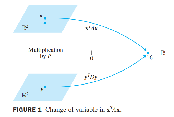
Change of Variable in a Quadratic Form
Let A be an $n \times n$ symmetric matrix. Then there is an orthogonal change of variable, $\vec{x} = P\vec{y}$, that transforms the quadratic form $\vec{x}^TA\vec{x}$ into a quadratic form $\vec{y}^TD\vec{y}$ with no cross-product term.
The columns of $P$ in the theorem are called the principal axes of the quadratic form(二次型的主轴) $\vec{x}^TA\vec{x}$. The vector $\vec{y}$ is the coordinate vector of $\vec{x}$ relative to the orthonormal basis of $R^n$ given by these principal axes.
💡For Example 💡:
Make a change of variable that transforms the quadratic form $Q(\vec{x}) = x_1^2 - 8x_1x_2 - 5x_2^2$ into a quadratic form with no cross-product term.
Solution:
The matrix of the quadratic form is
$$
A =
\begin{bmatrix}
1 & -4\\
-4 & -5
\end{bmatrix}
$$
The first step is to orthogonally diagonalize $A$.
$$
\lambda = 3 :
\begin{bmatrix}
2/\sqrt{5}\\
-1/\sqrt{5}
\end{bmatrix};
$$
$$
\lambda = -7 :
\begin{bmatrix}
1/\sqrt{5}\\
2/\sqrt{5}
\end{bmatrix}
$$
Let
$$
P = \begin{bmatrix}
2/\sqrt{5} & 1/\sqrt{5}\\
-1/\sqrt{5} & 2/\sqrt{5}
\end{bmatrix},
D = \begin{bmatrix}
3 & 0\\
0 & -7
\end{bmatrix}
$$
Then $A = PDP^{-1}$ and $D = P^{-1}AP = P^TAP$, as pointed out earlier. A suitable change of variable is
$$
\vec{x} = P\vec{y},
where \space \vec{x} =
\begin{bmatrix}
x_1 \\ x_2
\end{bmatrix}
and
\vec{y} =
\begin{bmatrix}
y_1\\
y_2
\end{bmatrix}
$$
Then,
$$
x_1^2 - 8x_1x_2 - 5x_2^2
= \vec{x}^TA\vec{x}
= (P\vec{y})^TA(P\vec{y})\\
= \vec{y}^TP^TAP\vec{y}
= \vec{y}^TD\vec{y}
= 3y_1^2-7y_2^2
$$
To illustrate the meaning of the equality of quadratic forms, we can compute $Q(\vec{x})$ for $\vec{x} = (2,-2)$ using the new quadratic form. First, since $\vec{x} = P\vec{y}$,
$$
\vec{y} = P^{-1}\vec{x} = P^T\vec{x}
$$
so,
$$
\vec{y} =
\begin{bmatrix}
2/\sqrt{5} & -1/\sqrt{5}\\
1/\sqrt{5} & 2/\sqrt{5}
\end{bmatrix}
\begin{bmatrix}
2\\-2
\end{bmatrix}=
\begin{bmatrix}
6/\sqrt{5} \\-2/\sqrt{5}
\end{bmatrix}
$$
Hence, $3y_1^2-7y_2^2 = 16$
A Geometric View of Principal Axes
$$
\vec{x}^TA\vec{x} = c, c : constant, A:symmetric \tag{3}
$$
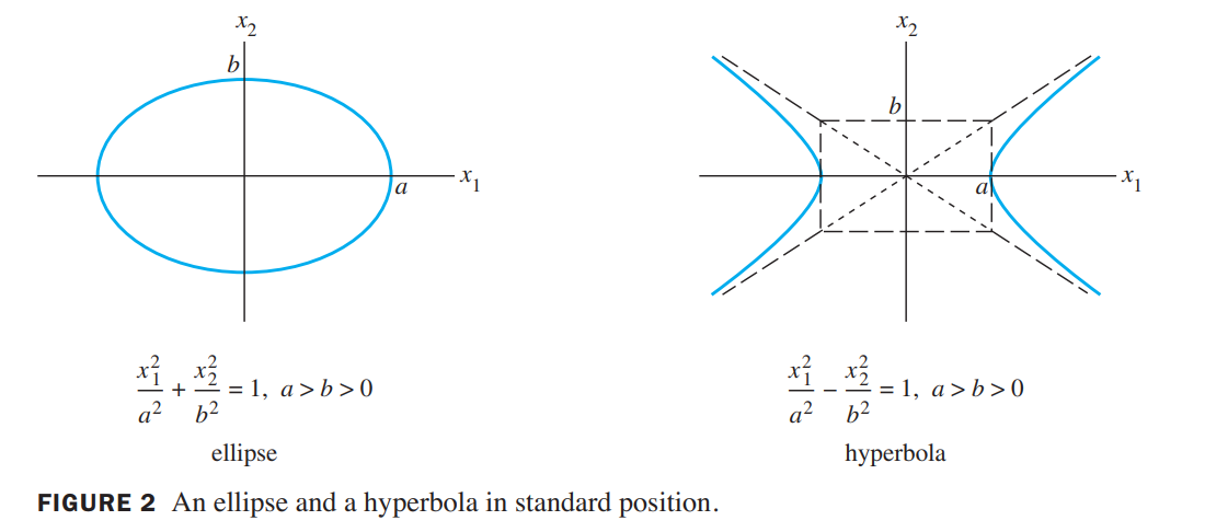
If $A$ is a diagonal matrix(对角矩阵), the graph is in standard position, such as in Figure 2.
If $A$ is not a diagonal matrix(不是对角矩阵), the graph of equation (3) is rotated out of standard position, as in Figure 3. Finding the principal axes (determined by the eigenvectors of $A$) amounts to finding a new coordinate system with respect to which the graph is in standard position.
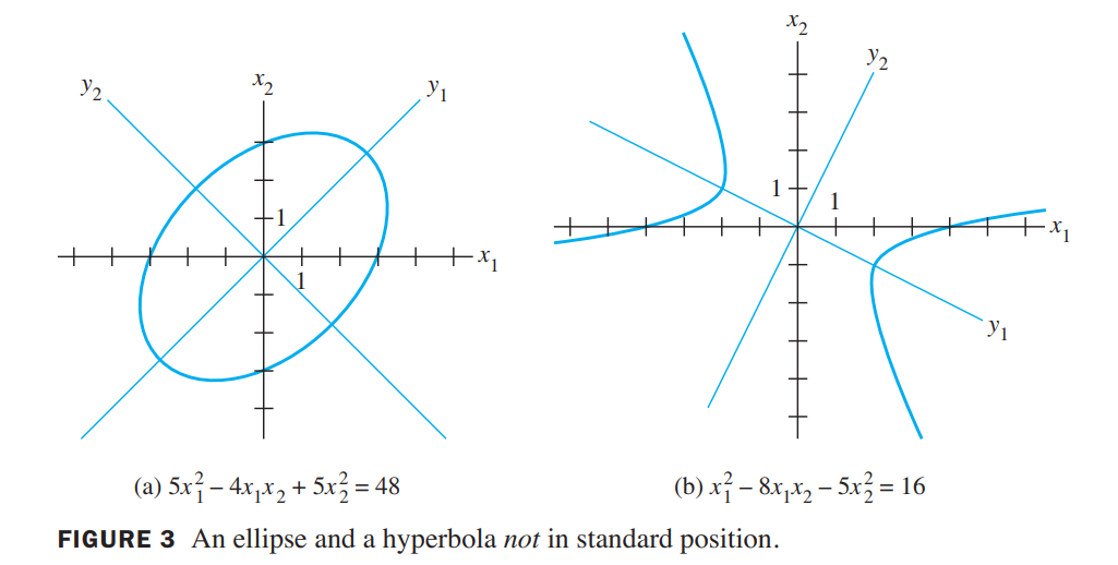
The hyperbola in Figure 3(b) is the graph of the equation $\vec{x}^TA\vec{x} = 16$, where $A$ is the matrix in above Example
$$
A =
\begin{bmatrix}
1 & -4\\
-4 & -5
\end{bmatrix}
$$
The positive $y_1-axis$ in Figure 3(b) is in the direction of the first column of the matrix $P$, and the positive $y_2-axis$ is in the direction of the second column of $P$ .
$$
P =
\begin{bmatrix}
2/\sqrt{5} & 1/\sqrt{5}\\
-1/\sqrt{5} & 2/\sqrt{5}
\end{bmatrix}
$$
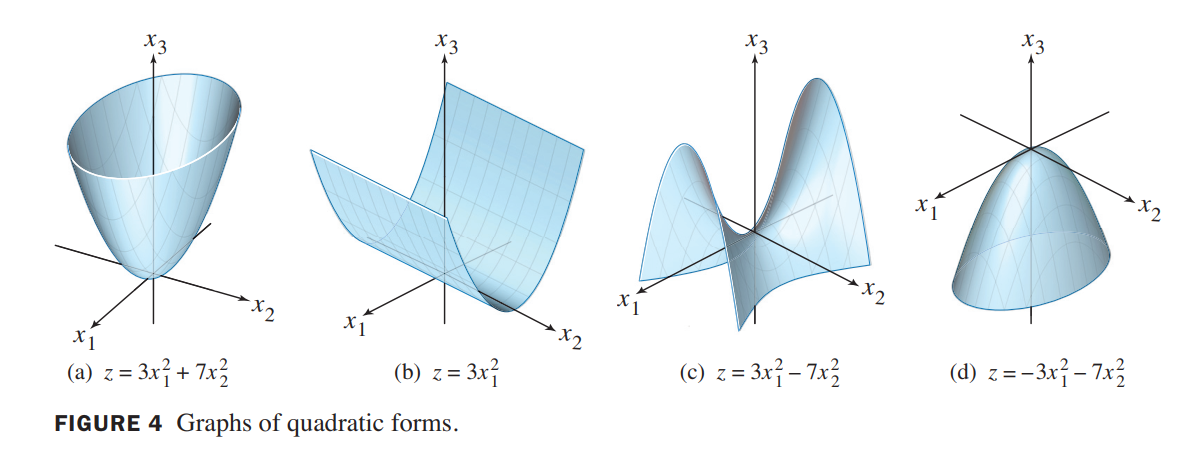
Classifying Quadratic Forms
A quadratic form $Q$ is:
a. positive definite(正定) if $Q(\vec{x}) > 0$ for all $\vec{x} \neq \vec{0}$
b. negative definite(负定) if $Q(\vec{x}) < 0$ for all $\vec{x} \neq \vec{0}$
c. indefinite if $Q(\vec{x})$ assumes both positive and negative values.
$Q(\vec{x})$ is said to be positive semidefinite if $Q(\vec{x}) \geq 0$ for all $\vec{x}$, and to be negative semidefinite if$Q(\vec{x}) \leq 0$ for all $\vec{x}$.
Let $A$ be an $n \times n$ symmetric matrix. Then a quadratic form $\vec{x}^TA\vec{x}$ is:
a. positive definite if and only if the eigenvalues of $A$ are all positive,
b. negative definite if and only if the eigenvalues of $A$ are all negative, or
c. indefinite if and only if $A$ has both positive and negative eigenvalues.
Constrained Optimization(有约束的优化)
When a quadratic form $Q$ has no cross-product terms, it is easy to find the maximum and minimum of $Q(\vec{x})$ for $\vec{x}^T\vec{x} = 1$.
💡Example1💡:
Find the maximum and minimum values of $Q(\vec{x}) = 9x_1^2 + 4x_2^2 + 3x_3^2$ subject to the constraint $\vec{x}^T\vec{x} = 1$.
Solution:
$$
\vec{x}^T\vec{x} = 1\iff ||\vec{x}|| = 1 \iff ||\vec{x}||^2 = 1 \iff x:unit-vector
$$
Since $x_2^2$ and $x_3^2$ are nonnegative, note that
$$
4x_2^2 \leq 9x_2^2, and \space 3x_3^2 \leq 9x_3^2
$$
hence,
$$
\begin{aligned}
Q(\vec{x}) &= 9x_1^2 + 4x_2^2 + 3x_3^2 \\
&\leq 9x_1^2 + 9x_2^2 + 9x_3^2 \\
&= 9
\end{aligned}
$$
So the maximum value of $Q(\vec{x})$ cannot exceed $9$ when $\vec{x}$ is a unit vector.
To find the minimum value of $Q(\vec{x})$, observe that
$$
9x_1^2 \geq 3x_1^2, and \space 4x_2^2 \geq 3x_2^2
$$
hence,
$$
\begin{aligned}
Q(\vec{x}) \geq 3x_1^2 + 3x_2^2 + 3x_3^2 = 3
\end{aligned}
$$
that the matrix of the quadratic form $Q(\vec{x})$ has eigenvalues $9, 4, and 3$ and that the greatest and least eigenvalues equal, respectively, the (constrained) maximum and minimum of $Q(\vec{x})$. The same holds true for any quadratic form, as we shall see.(最值和特征值相关)
💡Example2💡:
Let $A = \begin{bmatrix} 3 & 0 \\0 & 7\end{bmatrix}$, and let $Q(\vec{x}) = \vec{x}^TA\vec{x}$ for $\vec{x}$ in $R^2$. Figure 1 displays the graph of $Q$. Figure 2 shows only the portion of the graph inside a cylinder; the intersection of the cylinder with the surface is the set of points $(x_1,x_2,z)$such that $z = Q(x_1,x_2)$ and $x_1^2 + x_2^2 = 1$. Geometrically, the constrained optimization problem is to locate the highest and lowest points on the intersection curve.
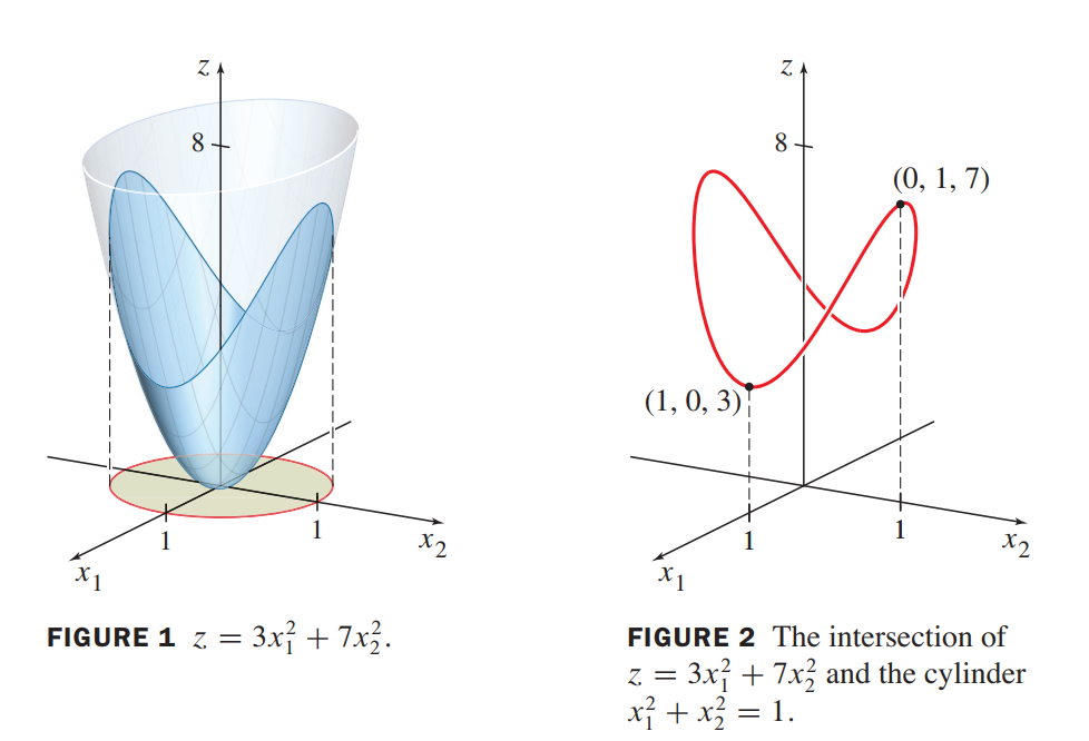
The two highest points on the curve are $7$ units above the $x_1x_2-plane$, occurring where $x_1 = 0$ and $x_2 = \pm 1$. These points correspond to the eigenvalue $7$ of $A$ and the eigenvectors $\vec{x} = (0, 1) and -\vec{x} = (0,-1)$. Similarly, the two lowest points on the curve are $3$ units above the $x_1x_2-plane$. They correspond to the eigenvalue $3$ and the eigenvectors $(1, 0) and (-1,0)$.
let
$$
m = min\lbrace \vec{x}^TA\vec{x} : ||\vec{x}|| = 1\rbrace\\
M = max\lbrace \vec{x}^TA\vec{x} : ||\vec{x}|| = 1\rbrace
\tag{2}
$$
Let $A$ be a symmetric matrix, and define $m$ and $M$ as in (2). Then $M$ is the greatest eigenvalue $\lambda_1$ of $A$ and $m$ is the least eigenvalue of $A$. The value of $\vec{x}^TA\vec{x}$ is $M$ when $\vec{x}$ is a unit eigenvector $\vec{u_1}$ corresponding to $M$. The value of $\vec{x}^TA\vec{x}$ is $m$ when $\vec{x}$ is a unit eigenvector corresponding to $m$.
Then the maximum value of $\vec{x}^TA\vec{x}$ subject to the constraints
$$
\vec{x}^T\vec{x} = 1, \vec{x}^T\vec{u_1} = 0
$$
is the second greatest eigenvalue, $\lambda_2$, and this maximum is attained when $\vec{x}$ is an eigenvector $\vec{u_2}$ corresponding to $\lambda_2$.
Let $A$ be a symmetric $n \times n$ matrix with an orthogonal diagonalization $A = PDP^{-1}$, where the entries on the diagonal of $D$ are arranged so that $\lambda_1 \geq \lambda_2 \geq \cdots \lambda_n$ and where the columns of $P$ are corresponding unit eigenvectors $\vec{u_1}, \cdots, \vec{u_n}$. Then for $k = 2, \cdots, n$, the maximum value of $x^TAx$ subject to the constraints
$$
\vec{x}^T\vec{x} = 1, \vec{x}^T\vec{u_1} = 0, \cdots, \vec{x}^T\vec{u_{k-1}} = 0
$$
is the eigenvalue $\lambda_k$, and this maximum is attained at $\vec{x} = \vec{u_k}$.
The Singular Value Decomposition
Unfortunately, as we know, not all matrices can be factored as $A = PDP^{-1}$ with $D$ diagonal. However, a factorization $A = QDP^{-1}$ is possible for any $m \times n$ matrix $A$. A special factorization of this type, called the singular value decomposition, is one of the most useful matrix factorizations in applied linear algebra.
The absolute values of the eigenvalues of a symmetric matrix A measure the amounts that A stretches or shrinks certain vectors (the eigenvectors).
For a symmetric $A$, if $A\vec{x} = \lambda \vec{x}$ and $||\vec{x}|| = 1$, then
$$
||A\vec{x}|| = ||\lambda \vec{x}|| = |\lambda| ||\vec{x}|| = |\lambda|
\tag{1}
$$
If $\lambda_1$ is the eigenvalue with the greatest magnitude, then a corresponding unit eigenvector $\vec{v_1}$ identifies a direction in which the stretching effect of $A$ is greatest. That is, the length of $A\vec{x}$ is maximized when $\vec{x} = \vec{v_1}$, and $A\vec{v_1} = \lambda_1$, by (1).
💡For example💡:
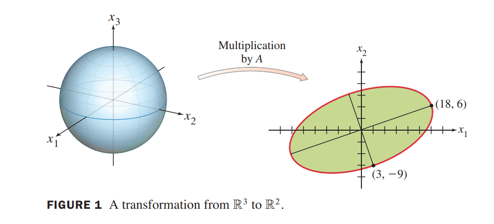
If $A = \begin{bmatrix}4 & 11 & 14\\8 & 7 & -2\end{bmatrix}$, then the linear transformation $\vec{x} \mapsto A\vec{x}$ maps the unit sphere $\lbrace \vec{x} : ||\vec{x}|| = 1\rbrace$ in $R^3$ onto an ellipse in $R^2$, shown in Figure 1. Find a unit vector $\vec{v}$ at which the length $||A\vec{x}||$ is maximized, and compute this maximum length.
Solution:
$$
||A\vec{x}||^2 = (A\vec{x})^T(A\vec{x}) = \vec{x}^T(A^TA)\vec{x}
$$
$A^TA$ is a symmetric matrix, So the problem now is to maximize the quadratic form $\vec{x}^T(A^TA)\vec{x}$ subject to the constraint $||\vec{x}|| = 1$.
The eigenvalues of $A^TA$ are $\lambda_1 = 360, \lambda_2 = 90, \lambda_3 = 0$. Corresponding unit eigenvectors are, respectively:
$$
\vec{v_1} = \begin{bmatrix}1/3 \\ 2/3 \\ 2/3\end{bmatrix},
\vec{v_2} = \begin{bmatrix}-2/3 \\ -1/3 \\ 2/3\end{bmatrix},
\vec{v_1} = \begin{bmatrix}2/3 \\ -2/3 \\ 1/3\end{bmatrix}
$$
The maximum value of $||A\vec{x}||^2$ is 360, The vector $A\vec{v_1}$ is a point on the ellipse in Figure 1 farthest from the origin, namely.
$$
A\vec{v_1} = \begin{bmatrix}18\\6\end{bmatrix}
$$
the maximum value of $A||\vec{x}||$ is $||A\vec{v_1}|| = \sqrt 360 = 6\sqrt 10$.
The Singular Values of an $m \times n$ Matrix
Let A be an $m \times n$ matrix. Then $A^TA$ is symmetric and can be orthogonally diagonalized. Let $\lbrace \vec{v_1}, \cdots, \vec{v_n}\rbrace$ be an orthonormal basis for $R^n$ consisting of eigenvectors of $A^TA$, and let $\lambda_1, \cdots, \lambda_n$ be the associated eigenvalues of $A^TA$. Then, for $1 \leq i \leq n$,
$$
\begin{aligned}
||A\vec{v_i}||^2 &= (A\vec{v_i})^TA\vec{v_i} = \vec{v_i}^TA^TA\vec{v_i}\\
&= \vec{v_i}^T(\lambda_i\vec{v_i})\\
&= \lambda_i
\end{aligned}
\tag{2}
$$
The singular values of $A$ are the square roots of the eigenvalues of $A^TA$, the singular values of $A$ are the lengths of the vectors $A\vec{v_1}, \cdots, A\vec{v_n}$.
The Singular Value Decomposition(奇异值分解)
The decomposition of $A$ involves an $m \times n$ “diagonal” matrix $\Sigma$ of the form
$$
\Sigma = \begin{bmatrix}
D & 0\\
0 & 0
\end{bmatrix}
\tag{3}
$$
where $D$ is an $r \times r$ diagonal matrix.
Let $A$ be an $m \times n$ matrix with rank $r$. Then there exists an $m \times n$ matrix $\Sigma$ as in (3) for which the diagonal entries in $D$ are the first $r$ singular values of $A$, $\sigma_1 \geq \sigma_2 \geq \cdots \geq \sigma_r > 0$, and there exist an $m \times m$ orthogonal matrix(正交矩阵) $U$ and an
$n \times n$ orthogonal matrix(正交矩阵) $V$ such that
$$
A = U \Sigma V^T
$$
but the diagonal entries of $\Sigma$ are necessarily the singular values of $A$.
The columns of $U$ in such a decomposition are called left singular vectors of $A$, and the columns of $V$ are called right singular vectors of A.
💡For example💡:
Construct a singular value decomposition of $A = \begin{bmatrix}4 & 11 & 14\\8 & 7 & -2\end{bmatrix}$
Solution:
Step1. Find an orthogonal diagonalization of $A^TA$.(find the eigenvalues of $A^TA$ and a corresponding orthonormal set of eigenvectors.)
Step2. Set up $V$ and $\Sigma$. Arrange the eigenvalues of $A^TA$ in decreasing order. The corresponding unit eigenvectors, $\vec{v_1}, \vec{v_2}, \vec{v_3}$, are the right singular vectors of $A$.
$$
V = \begin{bmatrix}
\vec{v_1} & \vec{v_2} & \vec{v_3}
\end{bmatrix}
=
\begin{bmatrix}
1/3 & -2/3 & 2/3\\
2/3 & -1/3 & -2/3\\
2/3 & 2/3 & 1/3
\end{bmatrix}
$$
The square roots of the eigenvalues are the singular values.
$$
\sigma_1 = 6\sqrt{10},
\sigma_2 = 3\sqrt{10},
\sigma_3 = 0
$$
The nonzero singular values are the diagonal entries of $D$.
$$
D = \begin{bmatrix}
6\sqrt 10 & 0\\
0 & 3\sqrt 10
\end{bmatrix}
\longrightarrow
\Sigma = \begin{bmatrix} D & 0\end{bmatrix}
= \begin{bmatrix}
6\sqrt 10 & 0 & 0\\
0 & 3\sqrt 10 & 0
\end{bmatrix}
$$
Step3. Construct $U$.
When A has rank $r$, the first $r$ columns of $U$ are the normalized vectors obtained from $A\vec{v_1}, \cdots, A\vec{v_r}$. In this example, $A$ has two nonzero singular values, so $rank A = 2$.
Recall from equation (2), $||A\vec{v_1}|| = \sigma_1, ||A\vec{v_2}|| = \sigma_2$. Thus
$$
\vec{u_1} = \frac{1}{\sigma_1}A\vec{v_1} =
\begin{bmatrix}
3/\sqrt 10\\1/\sqrt10
\end{bmatrix},
\vec{u_2} = \frac{1}{\sigma_2}A\vec{v_2} =
\begin{bmatrix}
1/\sqrt 10\\-3/\sqrt 10
\end{bmatrix}
$$
Thus,
$$
A =
\begin{bmatrix}
3/\sqrt 10 & 1/\sqrt 10\\ 1/\sqrt10 & -3/\sqrt 10
\end{bmatrix}
\begin{bmatrix}
6\sqrt 10 & 0 & 0\\
0 & 3\sqrt 10 & 0
\end{bmatrix}
\begin{bmatrix}
1/3 & -2/3 & 2/3\\
2/3 & -1/3 & -2/3\\
2/3 & 2/3 & 1/3
\end{bmatrix}
$$
Applications of the Singular Value Decomposition
The Invertible Matrix Theorem (concluded)
Let $A$ be an $n \times n$ matrix. Then the following statements are each equivalent to the statement that $A$ is an invertible matrix.
u. $(Col A)^\perp = {0}$.
v. $(Null A)^\perp = R^n$.
w. $RowA = R^n$.
x. $A$ has $n$ nonzero singular values.
💡For example💡:
Given the equation $Ax = b$, A is a $m \times n$ matrix, use the pseudoinverse of $A$ to define
$$
\hat{\vec{x}} = A^{\dagger}\vec{b} = V_rD^{-1}U_R^T\vec{b}
$$
where
$$
r = rank(A)
$$
👉More about SVD Decomposition by Numerical Analysis >>
Applications to Image Processing and Statistics
💡for example💡:
An example of two-dimensional data is given by a set of weights and heights of $N$ college students. Let $X_j$ denote the observation vector in $R^2$ that lists the weight and height of the $j th$ student. If $w$ denotes weight and $h$ height, then the matrix of observations has the form
$$
\begin{matrix}
w_1 & w_2 & \cdots & w_N\\
h_1 & h_2 & \cdots & h_N\\
\uparrow & \uparrow & &\uparrow\\
X_1 & X_2 & & X_N
\end{matrix}
$$
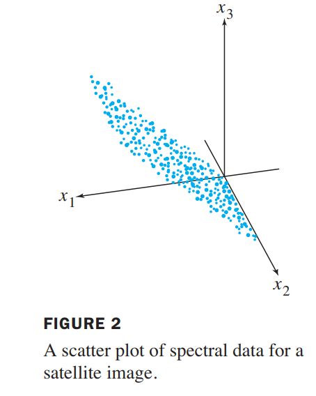
The set of observation vectors can be visualized as a two-dimensional scatter plot. See Figure 1.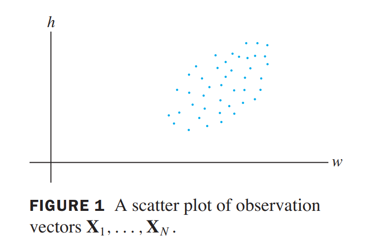
Mean and Covariance(均值和协方差)
let $\begin{bmatrix} X_1 \cdots X_N\end{bmatrix}$ be a $p \times N$ matrix of observations, such as described above. The sample mean, $M$, of the observation vectors $X_1 \cdots X_N$ is given by
$$
M = \frac{1}{N}(X_1 + \cdots + X_n)
$$
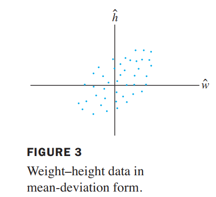
for $k = 1, \cdots, N$, let
$$
\hat{X_k} = X_k - M
$$
The columns of the $p \times N$ matrix
$$
B =
\begin{bmatrix}
\hat{X_1} \hat{X_2} \cdots \hat{X_N}
\end{bmatrix}
$$
have a zero sample mean, and B is said to be in mean-deviation form.
The (sample) covariance matrix is the $p \times p$ matrix $S$ defined by
$$
S = \frac{1}{N-1}BB^T
$$
Since any matrix of the form $BB^T$ is positive semidefinite, so is $S$.
💡For example💡:
Three measurements are made on each of four individuals in a random sample from a population. The observation vectors are
$$
X_1 = \begin{bmatrix} 1 \\ 2 \\ 1\end{bmatrix},
X_2 = \begin{bmatrix} 4 \\ 2 \\ 13\end{bmatrix},
X_3 = \begin{bmatrix} 7 \\ 8 \\ 1\end{bmatrix},
X_4 = \begin{bmatrix} 8 \\ 4 \\ 5\end{bmatrix}
$$
Compute the sample mean and the covariance matrix.
Solution:
$$
M = \begin{bmatrix}5 \\ 4 \\ 5\end{bmatrix},
B = \begin{bmatrix}4 & -1 & 2 & 3 \\ -2 & -2 & 4 & 0 \\ -4 & 8 & -4 & 0\end{bmatrix},
S = \begin{bmatrix}10 & 6 & 0 \\ 6 & 8 & -8 \\ 0 & -8 & 32\end{bmatrix}
$$
To discuss the entries in $S = [S_{ij}]$, denote the coordinates of $X$ by $x_1, \cdots, x_p$. For each $j = 1, \cdots, p$, the diagonal entry $s_{jj}$ in $S$ is called the variance of $x_j$. The variance of $x_j$ measures the spread of the values of $x_j$ .
The total variance of the data is the sum of the variances on the diagonal of $S$.
$$
\lbrace{total \space variance\rbrace} = tr(S)
$$
The entry $s_{ij}$ in $S$ for $i \neq j$ is called the covariance of $x_i$ and $x_j$.
(1,3)-entry in $S$ is $0$. Statisticians say that $x_1$ and $x_3$ are uncorrelated.
Principal Component Analysis(主成分分析)
Suppose the matrix $[X_1, \cdots, X_N]$ is already in mean-deviation form. The goal of principal component analysis is to find an orthogonal $p \times p$ matrix(正交矩阵) $P = [u_1 \cdots u_p]$ that determines a change of variable, $X = PY$, or
$$
\begin{bmatrix}
x_1 \\
x_2\\
\cdots \\
x_p
\end{bmatrix} =
\begin{bmatrix}
u_1 & u_2 & \cdots & u_p
\end{bmatrix}
\begin{bmatrix}
y_1 \\ y_2 \\ \cdots \\ y_p
\end{bmatrix}
$$
with the property that the new variables $y_1, \cdots, y_p$ are uncorrelated and are arranged in order of decreasing variance.
Recall the Quadratic form we learned above, $\vec{x} = P\vec{y}$, the columns of $P$ means the correspongding unit eigen vectors to eigen values(decreased) of $A$, so that, $Q = x^TAx = y^TDy, A = PDP^{-1} = PDP^T$, similar, Right?
Notice that $Y_k$ is the coordinate vector of $X_k$ with respect to the columns of $P$, and $Y_k = P^{-1}X_k = P^T X_k$ for $k = 1, \cdots, N$.
Thus, the covariance matrix of $Y_1, \cdots, Y_N$ is $D = P^TSP$. $D$ is a diagonal matrix.
The unit eigenvectors $u_1, \cdots, u_p$ of the covariance matrix $S$ are called the principal components of the data (in the matrix of observations). The first principal component is the eigenvector corresponding to the largest eigenvalue of $S$.
Thus $y_1$ is a linear combination of the original variables $x_1, \cdots, x_p$, using the entries in the eigenvector $u_1$ as weights.
$$
y_1 = u_1^TX = c_1x_1 + c_2x_2 + \cdots + c_px_p
$$
💡For example💡:
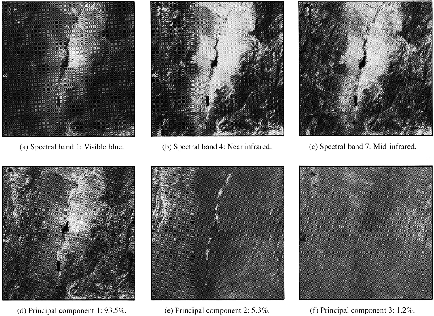
The initial data for the multispectral image of Railroad Valley consisted of 4 million vectors in $R^3$. The associated covariance matrix is
$$
S = \begin{bmatrix}
2382.78 & 2611.84 & 2136.20\\
2611.84 & 3106.47 & 2553.90\\
2136.20 & 2553.90 & 2650.71
\end{bmatrix}
$$
Find the principal components of the data, and list the new variable determined by the first principal component.
Solution:
$$
\lambda_1 = 7614.23, \lambda_1 = 427.63, \lambda_1 = 98.10, \\
$$
$$
\vec{u_1} = \begin{bmatrix} 0.5417 \\ 0.6295 \\ 0.5570\end{bmatrix},
\vec{u_2} = \begin{bmatrix} -0.4894 \\ -0.3026\\ 0.8179\end{bmatrix},
\vec{u_3} = \begin{bmatrix} 0.6834 \\ -0.7157 \\ 0.1441\end{bmatrix}
$$
the variable for the first principal component is
$$
y_1 = 0.54x_1 + 0.63x_2 + 0.56x_3
$$
This equation was used to create photograph (d) as follows. The variables $x_1, x_2, and x_3$ are the signal intensities in the three spectral bands.
At each pixel in photograph (d), the gray scale value is computed from $y_1$, a weighted linear combination of $x_1, x_2, and x_3$. In this sense, photograph (d) “displays” the first principal component of the data.
(Sensors aboard the satellite acquire seven simultaneous images of any region on earth to be studied. The sensors record energy from separate wavelength bands— three in the visible light spectrum and four in infrared and thermal bands.)
As we shall see, this fact will permit us to view the data as essentially one-dimensional rather than three-dimensional.
Reducing the Dimension of Multivariate Data
It can be shown that an orthogonal change of variables, $X = PY$, does not change the total variance of the data. (Roughly speaking, this is true because left-multiplication by $P$ does not change the lengths of vectors or the angles between them.)(正交矩阵的性质)
$$
\lbrace total \space variance \space of \space x_1, \cdots, x_p\rbrace
=
\lbrace total \space variance \space of \space y_1, \cdots, y_p\rbrace
=
\lambda_1 + \lambda_2 + \cdots + \lambda_p
$$
In a sense, 93.5%(7614.23/(7614.23+427.63+98.10)) of the information collected by Landsat for the Railroad Valley region is displayed in photograph (d), with 5.3% in (e) and only 1.2% remaining for (f). which means that the points lie approximately along a line, and the data are essentially one-dimensional.
Characterizations of Principal Component Variables
The singular value decomposition is the main tool for performing principal component analysis in practical applications.
if $B$ is a $p \times N$ matrix of observations in mean-deviation form, and if $A = (1/\sqrt{N-1})B^T$, then $A^TA$ is the covariance matrix $S$.
The squares of the singular values of $A$ are the $p$ eigenvalues of $S$.
The right singular vectors of $A$ are the principal components of the data.
Iterative calculation of the $SVD$ of $A$ is faster and more accurate than an eigenvalue decomposition of $S$.

