Keywords: Least Squares, QR Factorization, Levenberg–Marquardt Method, Gauss–Newton Method, Mathlab
Least Squares and the Normal Equations
Why Least Squares?
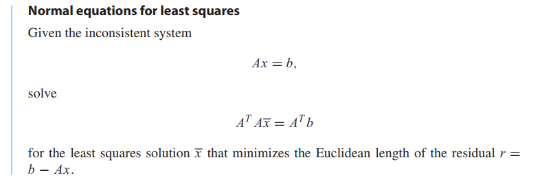
- For Chapter2, get the solution of $Ax = b$, what if there’s no Solution? When the equations are inconsistent, which is likely if the number of equations exceeds the number of unknowns, the answer is to find the next best thing: the least squares approximation.
- For Chapter3, find the polynomials to fit data points. However, if the data points are numerous, or the data points are collected only within some margin of error, fitting a high-degree polynomial exactly is rarely the best approach. In such cases, it is more reasonable to fit a simpler model that may only approximate the data points.
👉More about Least Squares in Algebra >>
Inconsistent systems of equations
A system of equations with no solution is called inconsistent.
There are at least three ways to express the size of the residual.
The Euclidean length of a vector,
$$
||r||_2 = \sqrt{r_1^2 + r_2^2 + \cdots + r_m^2}
\tag{4.7}
$$
is a norm, called the 2-norm.
The squared error,
$$
SE = r_1^2 + r_2^2 + \cdots + r_m^2
$$
and the root mean squared error (the root of the mean of the squared error)
$$
RMSE = \sqrt{SE/m} = \frac{||r||_2}{\sqrt m}
\tag{4.8}
$$
Fitting models to data
Fitting data by least squares
STEP 1. Choose a model.
STEP 2. Force the model to fit the data.
STEP 3. Solve the normal equations.
Usually, the reason for using least squares is to replace noisy data with a plausible underlying model.The model is then often used for signal prediction or classification purposes.
We have presented the normal equations as the most straightforward approach to solving the least squares problem, and it is fine for small problems.However, the condition number $cond(A^TA)$ is approximately the square of the original $cond(A)$, which will greatly increase the possibility that the problem is ill-conditioned. More sophisticated methods allow computing the least squares solution directly from $A$ without forming $A^TA$. These methods are based on the QR-factorization, introduced in Section 4.3, and the singular value decomposition of Chapter 12.
Conditioning of least squares
💡For example💡:
Let $x_1 = 2.0,x_2 = 2.2,x_3 = 2.4, . . . , x_{11} = 4.0$ be equally spaced points in $[2,4]$, and set $y_i = 1 + x_i + x^2_i + x^3_i + x^4_i + x^5_i + x^6_i + x^7_i$ for $1 \leq i \leq 11$. Use the normal equations to find the least squares polynomial $P(x) = c_1 + c_2x + · · · + c_8x^7$ fitting the $(x_i,y_i)$.
Solution:
A degree $7$ polynomial is being fit to $11$ data points lying on the degree $7$ polynomial $P(x) = 1 + x + x^2 + x^3 + x^4 + x^5 + x^6 + x^7$.
$$
\begin{bmatrix}
1 & x_1 & x_1^2 & \cdots & x_1^7\\
1 & x_2 & x_2^2 & \cdots & x_2^7\\
& & \cdots &\\
1 & x_{11} & x_{11}^2 & \cdots & x_{11}^7
\end{bmatrix}
\begin{bmatrix}
c_1\\c_2\\ \cdots \\c_8
\end{bmatrix}
=
\begin{bmatrix}
y_1\\y_2\\ \cdots \\y_{11}
\end{bmatrix}
$$
The coefficient matrix $A$ is a Van der Monde matrix.
1 | >> x = (2+(0:10)/5)'; |
The value in my experiment is not the same with the book, so far I can’t find the reason…
Obviously, The condition number of $A^TA$ is too large to deal with in double precision arithmetic, and the normal equations are ill-conditioned, even though the original
least squares problem is moderately conditioned.
A Survey of Models
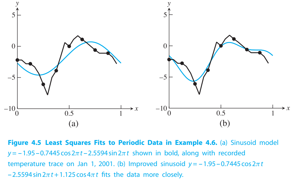
Periodic data
Periodic data calls for periodic models.Outside air temperatures, for example, obey cycles on numerous timescales, including daily and yearly cycles governed by the rotation of the earth and the revolution of the earth around the sun.
Data linearization
Exponential growth of a population is implied when its rate of change is proportional to its size.
The exponential model
$$
y = c_1e^{c_2t}
\tag{4.10}
$$
cannot be directly fit by least squares $Ax = b$ because $c_2$ does not appear linearly in the model equation.
Two methods to solve this problem. 1. Linearization thie nonlinear problem. 2. use nonlinear techniques, like Gauss-Newton Method, which will introduce next.
$$
\ln y = \ln(c_1e^{c_2t}) = \ln c_1 + \ln^{e^{c_2t}} = \ln c_1 + c_2 t
\tag{4.11}
$$
The $c_2$ coefficient is now linear in the model, but $c_1$ no longer is. By renaming $k = \ln c_1$, we can write
$$
\ln y = k + c_2 t
\tag{4.12}
$$
Now both coefficients $k$ and $c_2$ are linear in the model.
The original problem and the linearization problem, these are two different minimizations and have different solutions, meaning that they generally result in different values of the coefficients $c_1,c_2$. When you choose the techniques, choose the more natural choice.
💡For example💡:
Use model linearization to find the best least squares exponential fit $y = c_1e^{c_2t}$ to the following world automobile supply data:
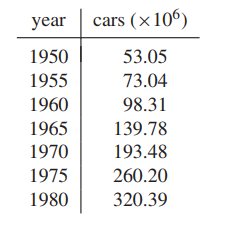
Solution:
$$
k_1 \approx 3.9896, c_2 \approx 0.06152, c_1 = e^{3.9896} \approx 54.03
$$
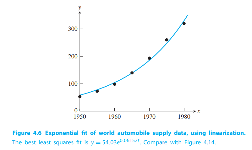
the RMSE of the log-linearized model in log space is $\approx 0.0357$, while RMSE of the original exponential model is $\approx 9.56$.
QR Factorization
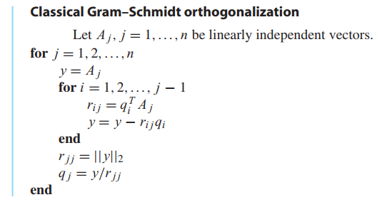
Gram–Schmidt orthogonalization and least squares
The result of Gram–Schmidt orthogonalization can be written in matrix form as, let A be $m \times n$ matrix.
$$
(A_1|\cdots|A_n) = (q_1|\cdots|q_n)
\begin{bmatrix}
r_{11} & r_{12} & \cdots & r_{1n}\\
& r_{22} & \cdots & r_{2n}\\
& & \ddots & \vdots\\
& & & r_{nn}
\end{bmatrix}
\tag{4.26}
$$
where, $r_{jj} = ||y_j||2$ and $r{ij} = q_i^TA_j$. Like
$$
y_1 = A_1, q_1 = \frac{y_1}{||y_1||_2}
\tag{4.23}
$$
$$
y_2 = A_2 - q_1(q_1^TA_2), q_2 = \frac{y_2}{||y_2||_2}
\tag{4.24}
$$
We call this $A = QR$ the reduced QR factorization.
This matrix equation is the full QR factorization:
$$
(A_1|\cdots|A_n) = (q_1|\cdots|q_m)
\begin{bmatrix}
r_{11} & r_{12} & \cdots & r_{1n}\\
& r_{22} & \cdots & r_{2n}\\
& & \ddots & \vdots\\
& & & r_{nn}\\
0 & \cdots & \cdots & 0\\
\vdots & & & \vdots\\
0 & \cdots & \cdots & 0\\
\end{bmatrix}
\tag{4.27}
$$
DEFINITION 4.1
A square matrix $Q$ is orthogonal if $Q^T = Q^{−1}$.
The key property of an orthogonal matrix is that it preserves the Euclidean norm of a vector.
LEMMA 4.2
If $Q$ is an orthogonal $m \times m$ matrix and $x$ is an $m$-dimensional vector, then $||Qx||_2 = ||x||_2$.
Proof.
$$
||Qx||_2^2 = (Qx)^T(Qx) = x^TQ^TQx = x^Tx = ||x||_2^2
$$
Doing calculations with orthogonal matrices is preferable because (1) they are easy to invert by definition,and (2) by Lemma4.2,they do not magnify errors.
There are three ways to use $QR$ factorization.
Sovle $Ax = b$. The $QR$ factorization of an $m \times m$ matrix by the Gram–Schmidt method requires approximately $m^3$ multiplication/divisions, three times more than the $LU$ factorization, plus about the same number of additions.
Calculate eigenvalues, which will be introduced in Chapter12.
Solve Least squares.
Let A be an $m \times n$ matrix, $m > n$. To minimize $||Ax - b||_2$, rewrite as $||QRx - b||_2 = ||Rx - Q^Tb||_2$ by lemma 4.2.
The vector inside the Euclidean norm is
$$
\begin{bmatrix}
e_1\\ \vdots \\ e_n \\ \hdashline \\ e_{n+1} \\ \vdots
\end{bmatrix}
=
\begin{bmatrix}
r_{11} & r_{12} & \cdots & r_{1n}\\
& r_{22} & \cdots & r_{2n}\\
& & \ddots & \vdots\\
& & & r_{nn}\\
0 & \cdots & \cdots & 0\\
\vdots & & & \vdots\\
0 & \cdots & \cdots & 0\\
\end{bmatrix}
\begin{bmatrix}
x_1\\ \vdots \\ x_n
\end{bmatrix}
-
\begin{bmatrix}
d_1 \\ \vdots \\ d_n \\ \hdashline \\ d_{n+1} \\ \vdots \\ d_m
\end{bmatrix}
\tag{4.28}
$$
the least squares solution is minimized by using the $x$ from back-solving the upper part, and
the least squares error is $||e||2^2 = d{n+1}^2 + \cdots + d^2_m$.
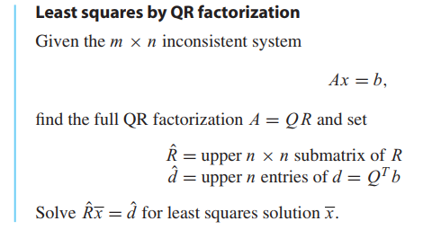
💡For example💡:
Use the full $QR$ factorization to solve the least squares problem
$$
\begin{bmatrix}
1 & -4\\
2 & 3\\
2 & 2
\end{bmatrix}
\begin{bmatrix}
x_1 \\ x_2
\end{bmatrix}
=
\begin{bmatrix}
-3\\ 15\\ 9
\end{bmatrix}
$$
Solution:
$$
Rx = Q^Tb
$$
$$
\begin{bmatrix}
3 & 2\\
0 & 5\\
\hdashline
0 & 0
\end{bmatrix}
\begin{bmatrix}
x_1 \\ x_2
\end{bmatrix}
=
\begin{bmatrix}
15\\ 9 \\ \hdashline 3
\end{bmatrix}
$$
The least squares error will be $||e||_2 = ||(0,0,3)||_2 = 3$. Equating the upper parts yields
$$
\begin{bmatrix}
3 & 2\\
0 & 5
\end{bmatrix}
\begin{bmatrix}
x_1 \\ x_2
\end{bmatrix}
=
\begin{bmatrix}
15\\ 9
\end{bmatrix}
$$
whose solution is
$$
\bar{x_1} = 3.8, \bar{x_2} = 1.8
$$
1 | >> x = (2+(0:10)/5)'; |
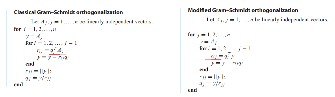
Modified Gram–Schmidt orthogonalization
A slight modification to Gram–Schmidt turns out to enhance its accuracy in machine calculations.
Householder reflectors
LEMMA 4.3
Assume that $x$ and $w$ are vectors of the same Euclidean length, $||x||_2 = ||w||_2$. Then $w − x$ and $w + x$ are perpendicular.
THEOREM 4.4
Householder reflectors. Let $x$ and $w$ be vectors with $||x||_2 = ||w||_2$ and define $v = w − x$. Then $H = I − 2vv^T / v^Tv$ is a symmetric orthogonal matrix and $Hx = w$.
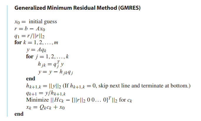
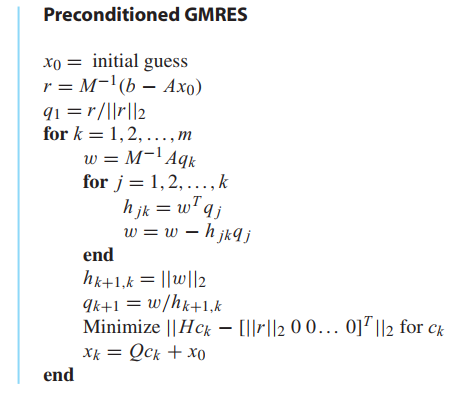
4.4 Generalized Minimum Residual (GMRES) Method
Krylov methods
Preconditioned GMRES
Nonlinear Least Squares
Gauss–Newton Method
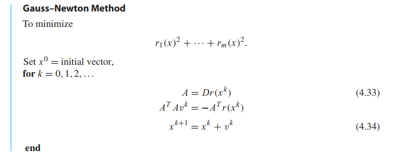
Models with nonlinear parameters
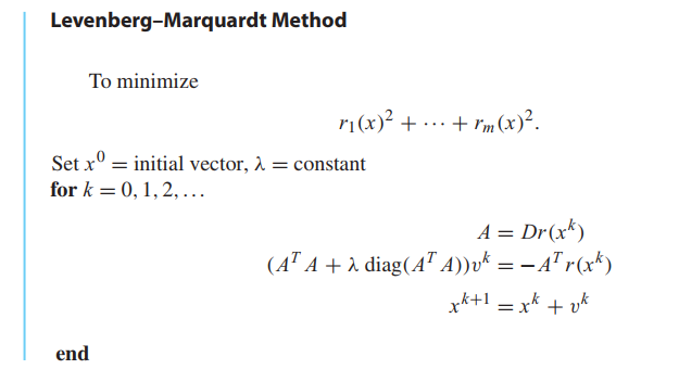
The Levenberg–Marquardt Method(LM Algorithm)
Reality Check 4: GPS,Conditioning, and Nonlinear Least Squares
to be added..

