Keywords: Orthogonal Projections, Gram-Schmidt Process, Least-Squares Problems, Linear Model
This is the Chapter6 ReadingNotes from book Linear Algebra and its Application.
The Inner Product
inner product is dot product.
$$
\vec{u}^T\vec{v} = \vec{u} \cdot \vec{v}
$$
The Length of a Vector
The length (or norm) of $\vec{v}$ is the nonnegative scalar $||\vec{v}||$ defined by
$$
||\vec{v}|| = \sqrt{\vec{v} \cdot \vec{v}} = \sqrt{v_1^2 + \cdots + v_n^2}
$$
Distance in $R^n$
$$
dis(\vec{u}, \vec{v}) = ||\vec{u} - \vec{v}||
$$
Orthogonal Vectors
$$
\vec{u} \cdot \vec{v} = 0
\Leftrightarrow
||\vec{u}+\vec{v}||^2 = ||\vec{u}||^2 + ||\vec{v}||^2
$$
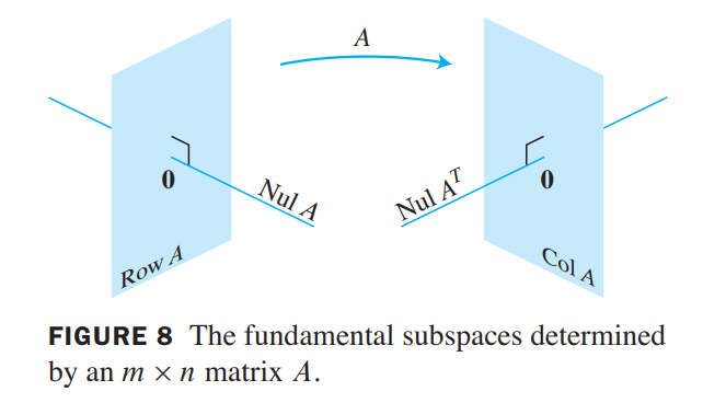
Orthogonal Complements
Let $A$ be an $m \times n$ matrix. The orthogonal complement of the row space of $A$ is the null space of $A$, and the orthogonal complement of the column space of $A$ is the null space of $A^T$ :
$$
(Row A)^\bot = NullA\\
(Col A)^\bot = NulA^T
$$
Angles in $R^2$ and $R^3$
$$
\vec{u} \cdot \vec{v} = ||\vec{u}|| ||\vec{v}|| \cos \theta
$$
Orthogonal Sets
Let $\lbrace \vec{u_1}, \cdots, \vec{u_p}\rbrace$ be an orthogonal basis(orthogonal $\neq$ orthonormal) for a subspace $W$ of $R^n$. For each $\vec{y}$ in $W$, the weights in the linear combination
$$
\vec{y} = c_1\vec{u_1} + \cdots + c_p\vec{u_p}
$$
are give by
$$
c_j = \frac{\vec{y} \cdot \vec{u_j}}{\vec{u_j} \cdot \vec{u_j}}
$$
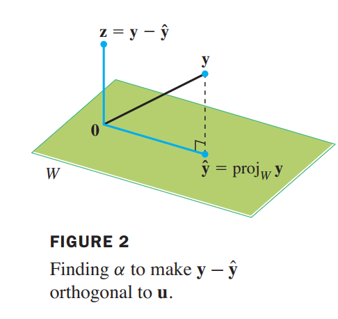
An Orthogonal Projection
Given a nonzero vector $\vec{u}$ in $R^n$, consider the problem of decomposing a vector $\vec{y}$ in $R^n$ into the sum of two vectors, one a multiple of $u$ and the other orthogonal to $u$. We wish to write
$$
\vec{y} = \hat{\vec{y}} + \vec{z}
$$
where $\hat{\vec{y}} = \alpha \vec{u}$ for some scalar $\alpha$˛ and $\vec{z}$ is some vector orthogonal to $\vec{u}$.
$$
\vec{z} \cdot \vec{u} = 0
\Rightarrow
(\vec{y} - \alpha \vec{u}) \cdot \vec{u} = 0\\
\Rightarrow
\alpha = \frac{\vec{y}\cdot \vec{u}}{\vec{u}\cdot\vec{u}}
,\hat{\vec{y}} = \frac{\vec{y}\cdot \vec{u}}{\vec{u}\cdot\vec{u}}\vec{u}
$$
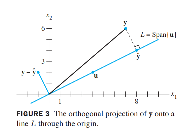
that means:
subspace $L$ spanned by $\vec{u}$ (the line through $\vec{u}$ and $\vec{0}$)
$$
\hat{\vec{y}} = proj_L\vec{y} = \frac{\vec{y}\cdot \vec{u}}{\vec{u}\cdot\vec{u}}\vec{u}
$$
Orthonormal Sets
A set $\lbrace \vec{u_1}, \cdots, \vec{u_p}\rbrace$ is an orthonormal set if it is an orthogonal set of unit vectors. If $W$ is the subspace spanned by such a set, then $\lbrace \vec{u_1}, \cdots, \vec{u_p}\rbrace$ is an orthonormal basis for $W$ , since the set is automatically linearly independent.
(正交矩阵)
An $m \times n$ matrix $U$ has orthonormal columns if and only if $U^TU = I$.
Let $U$ be an $m \times n$ matrix with orthonormal columns, and let $\vec{x}$ and $\vec{y}$ be in $R^n$. Then
a.$||U\vec{x}|| = ||\vec{x}||$转换保留长度和正交性
b.$(U\vec{x})\cdot (U\vec{y}) = \vec{x}\cdot \vec{y}$
c.$(U\vec{x})\cdot (U\vec{y}) = 0 ,if \space and \space only \space if,\vec{x}\cdot \vec{y} = 0$
Orthogonal Projections
Let $W$ be a subspace of $R^n$, let $\vec{y}$ be any vector in $R^n$, and let $\hat{\vec{y}}$ be the orthogonal projection of $\vec{y}$ onto $W$ . Then $\hat{\vec{y}}$ is the closest point in $W$ to $\vec{y}$, in the sense that
$$
||\vec{y}-\hat{\vec{y}}|| < ||\vec{y}-\vec{v}||
$$
for all $\vec{v}$ in $W$ distinct from $\hat{\vec{y}}$.
If $\lbrace \vec{u_1}, \cdots, \vec{u_p}\rbrace$ is an orthonormal basis for a subspace $W$ of $R^n$, then
$$
proj_W\vec{y} = (\vec{y} \cdot \vec{u_1})\vec{u_1} + \cdots + (\vec{y} \cdot \vec{u_p})\vec{u_p}
$$
if $U = \begin{bmatrix} \vec{u_1} & \vec{u_2} & \vec{u_p} \end{bmatrix}$, then
$$
proj_W\vec{y} = UU^T\vec{y}
$$
The Gram–Schmidt Process(构建标准正交基)
💡For Example💡:
Let $\vec{x_1} = \begin{bmatrix}1 \\ 1 \\1 \\1\end{bmatrix},\vec{x_2} = \begin{bmatrix}0 \\ 1 \\1 \\1\end{bmatrix},\vec{x_3} = \begin{bmatrix}0 \\ 0 \\1 \\1\end{bmatrix}$. Then $\lbrace \vec{x_1}, \vec{x_2}, \vec{x_3}\rbrace$ is clearly linearly independent and thus is a basis for a subspace $W$ of $R^4$. Construct an orthogonal basis for $W$ .
Solution:
Step 1. Let $\vec{v_1} = \vec{x_1}$ and $W_1 = Span \lbrace \vec{x_1} \rbrace =Span \lbrace \vec{v_1} \rbrace$.
Step 2. Let $\vec{v_2}$ be the vector produced by subtracting from $\vec{x_2}$ its projection onto the subspace $W_1$. That is, let
$$
\vec{v_2} = \vec{x_2} - proj_{W_1}\vec{x_2}
\\= \vec{x_2} - \frac{\vec{x_2} \cdot \vec{v_1}}{\vec{v_1} \cdot \vec{v_1}} \vec{v_1}
\\=
\begin{bmatrix}
-\frac{3}{4}\\
\frac{1}{4}\\
\frac{1}{4}\\
\frac{1}{4}
\end{bmatrix}
$$
$\lbrace \vec{v_1}, \vec{v_2}\rbrace$ is an orthogonal basis for the subspace $W_2$ spanned by $\vec{x_1}$ and $\vec{x_2}$ .
Step 2 (optional). If appropriate, scale $\vec{v_2}$ to simplify later computations. Since $\vec{v_2}$ has fractional entries, it is convenient to scale it by a factor of $4 $and replace $\lbrace \vec{v_1}, \vec{v_2}\rbrace$ by the orthogonal basis:
$$
\vec{v_1} = \begin{bmatrix}1 \\ 1 \\1 \\1\end{bmatrix},
\vec{v_2} = \begin{bmatrix}-3 \\ 1 \\1 \\1\end{bmatrix}
$$
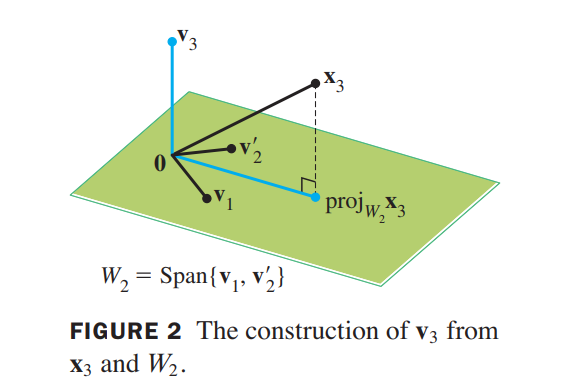
Step 3. Let $\vec{v_3}$ be the vector produced by subtracting from $\vec{v_3}$ its projection onto the subspace $W_2$. Use the orthogonal basis $\lbrace \vec{v_1}, \vec{v_2}\rbrace$ to compute this projection onto $W_2$:
$$
proj_{W_2}\vec{x_3} =
\frac{\vec{x_3} \cdot \vec{v_1}}{\vec{v_1} \cdot \vec{v_1}} \vec{v_1} +
\frac{\vec{x_3} \cdot \vec{v_2}}{\vec{v_2} \cdot \vec{v_2}} \vec{v_2},
\vec{v_3} = \vec{x_3} - proj_{W_2}\vec{x_3}
=
\begin{bmatrix}
0\\
\frac{-2}{3}\\
\frac{1}{3}\\
\frac{1}{3}
\end{bmatrix}
$$
$\lbrace \vec{v_1}, \vec{v_2}, \vec{v_3}\rbrace$ is an orthogonal basis for $W$ .
QR Factorization of Matrices
If $A$ is an $m \times n$ matrix with linearly independent columns, then $A$ can be factored as $A = QR$, where $Q$ is an $m \times n$ matrix whose columns form an orthonormal basis for $Col A$ and $R$ is an $n \times n$ upper triangular invertible matrix with positive entries on its diagonal.
💡For Example💡:
Find a $QR$ factorization of $A = \begin{bmatrix} 1 & 0 & 0\\1 & 1 & 0\\1 & 1 & 1\\1 & 1 & 1 \end{bmatrix}$.
Solution:
An orthogonal basis for $ColA = Span\lbrace \vec{x_1}, \vec{x_2}, \vec{x_3}\rbrace$ was found by Gram–Schmidt Process:
$$
\vec{v_1} = \begin{bmatrix}1 \\ 1 \\1 \\1\end{bmatrix},
\vec{v_2} = \begin{bmatrix}-3 \\ 1 \\1 \\1\end{bmatrix},
\vec{v_3} =
\begin{bmatrix}
0\\
\frac{-2}{3}\\
\frac{1}{3}\\
\frac{1}{3}
\end{bmatrix}
$$
Then normalize the three vectors to obtain $\vec{u_1}, \vec{u_2}, \vec{u_3}$, and use these vectors as the columns of $Q$:
$$
Q =
\begin{bmatrix}
\frac{1}{2} & \frac{-3}{\sqrt{12}} & 0 \\
\frac{1}{2} & \frac{1}{\sqrt{12}} & \frac{-2}{\sqrt{6}}\\
\frac{1}{2} & \frac{1}{\sqrt{12}} & \frac{1}{\sqrt{6}}\\
\frac{1}{2} & \frac{1}{\sqrt{12}} & \frac{1}{\sqrt{6}}
\end{bmatrix}
$$
because:
$$
Q^TA = Q^T(QR) = R
$$
thus:
$$
R = Q^TA =
\begin{bmatrix}
2 & \frac{3}{2} & 1 \\
0 & \frac{3}{\sqrt{12}} & \frac{2}{\sqrt{12}} \\
0 & 0 & \frac{2}{\sqrt{6}} \\
\end{bmatrix}
$$
👉More About LU Factorization >>
Least-Squares Problems(最小二乘问题)
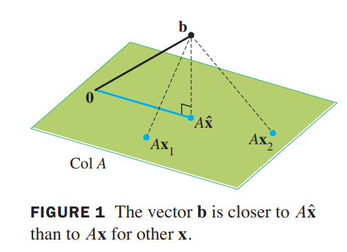
For $A\vec{x} = \vec{b}$, when a solution is demanded and none exists, the best one can do is to find an $\vec{x}$ that makes $A\vec{x}$ as close as possible to $\vec{b}$.
The general least-squares problem is to find an $\vec{x}$ that makes $||\vec{b} - A\vec{x}||$ as small as possible.
The adjective “least-squares” arises from the fact that $||\vec{b} - A\vec{x}||$ is the square root of a sum of squares(平方和的平方根).
If A is $m \times n$ and $\vec{b}$ is in $R^m$, a least-squares solution of $A\vec{x} = \vec{b}$ is an $\hat{x}$ in $R^n$such that
$$
||\vec{b} - A\hat{\vec{x}}|| \leq ||\vec{b} - A\vec{x}||
$$
for all $\vec{x}$ in $R^n$.
The most important aspect of the least-squares problem is that no matter what $\vec{x}$ we select, the vector $A\vec{x}$ will necessarily be in the column space $ColA$. So we seek an $\vec{x}$ that makes $A\vec{x}$ the closest point in $Col A$ to $\vec{b}$. See Figure 1. (Of course, if $\vec{b}$ happens to be in $Col A$, then $\vec{b}$ is $A\vec{x}$ for some $\vec{x}$, and such an $\vec{x}$ is a “least-squares solution.”)
Solution of the General Least-Squares Problem
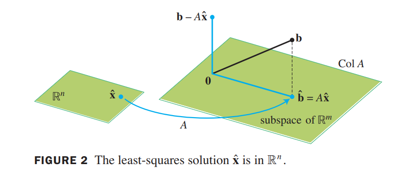
$$
\hat{\vec{b}} = proj_{ColA}\vec{b}
$$
Because $\hat{\vec{b}}$ is in the column space of $A$, the equation $A\vec{x} = \hat{\vec{b}}$ is consistent, and there is an $\hat{\vec{x}}$ in $R^n$ such that
$$
A\hat{\vec{x}} = \hat{\vec{b}}
$$
Since $\hat{\vec{b}}$ is the closest point in $Col A$ to $\vec{b}$, a vector $\hat{\vec{x}}$ is a least-squares solution of $A\vec{x} = \vec{b}$.
Suppose $\hat{\vec{x}}$ satisfies$A\hat{\vec{x}} = \hat{\vec{b}}$. The projection $\hat{\vec{b}}$ has the property that $\vec{b} - \hat{\vec{b}}$ is orthogonal to $Col A$. so $\vec{b} - \hat{\vec{b}}$ is orthogonal to each column of $A$. If $\vec{a_j}$ is any column of $A$, then $\vec{a_j}\cdot (\vec{b} - A\hat{\vec{x}}) = 0$, and $\vec{a_j}^T(\vec{b} - A\hat{\vec{x}}) = 0$(one is vector dot, one is matrix multiplication). Since each $\vec{a_j}^T$ is a row of $A^T$,
$$
A^T(\vec{b} - A\hat{\vec{x}}) = \vec{0}\tag{2}
\Rightarrow
A^T\vec{b} - A^TA\hat{\vec{x}} = \vec{0}
\Rightarrow
A^T\vec{b} = A^TA\hat{\vec{x}}
$$
These calculations show that each least-squares solution of $A\vec{x} = \vec{b}$ satisfies the equation
$$
A^TA\vec{x} = A^T\vec{b}\tag{3}
$$
The matrix equation (3) represents a system of equations called the normal equations(正规方程) for $A\vec{x} = \vec{b}$. A solution of (3) is often denoted by $\hat{\vec{x}}$.
💡For Example💡:
Find a least-squares solution of $A\vec{x} = \vec{b}$ for
$$
A =
\begin{bmatrix}
1 & 1 & 0 & 0\\
1 & 1 & 0 & 0\\
1 & 0 & 1 & 0\\
1 & 0 & 1 & 0\\
1 & 0 & 0 & 1\\
1 & 0 & 0 & 1\\
\end{bmatrix},
\vec{b} =
\begin{bmatrix}
-3\\-1\\0\\2\\5\\1
\end{bmatrix}
$$
Solution:
$$
A^TA =
\begin{bmatrix}
6 & 2 & 2 & 2\\
2 & 2 & 0 & 0\\
2 & 0 & 2 & 0\\
2 & 0 & 0 & 2\\
\end{bmatrix},
A^T\vec{b} =
\begin{bmatrix}
4\\-4\\2\\6
\end{bmatrix}
$$
The augmented matrix for $A^TA\vec{x} = A^T\vec{b}$ is
$$
\begin{bmatrix}
6 & 2 & 2 & 2 & 4\\
2 & 2 & 0 & 0 & -4\\
2 & 0 & 2 & 0 & 2\\
2 & 0 & 0 & 2 & 6\\
\end{bmatrix}
\sim
\begin{bmatrix}
6 & 2 & 2 & 2 & 4\\
2 & 2 & 0 & 0 & -4\\
2 & 0 & 2 & 0 & 2\\
2 & 0 & 0 & 2 & 6\\
\end{bmatrix}
\Rightarrow
\hat{\vec{x}} =
\begin{bmatrix}
3\\-5\\-2\\0
\end{bmatrix} + x_4
\begin{bmatrix}
-1\\1\\1\\1
\end{bmatrix}
$$
Let A be an $m \times n$ matrix. The following statements are logically equivalent:
a. The equation $A\vec{x} = \vec{b}$ has a unique least-squares solution for each $\vec{b}$ in $R^m$.
b. The columns of $A$ are linearly independent.
c. The matrix $A^TA$ is invertible.
When these statements are true, the least-squares solution $\hat{\vec{x}}$ is given by
$$
\hat{\vec{x}} = (A^TA)^{-1}A^T\vec{b}
$$
Alternative Calculations of Least-Squares Solutions
Given an $m \times n$ matrix $A$ with linearly independent columns, let $A = QR$ be a $QR$ factorization of $A$. Then, for each $\vec{b}$ in $R^m$, the equation $A\vec{x} = \vec{b}$ has a unique least-squares solution, given by
$$
\hat{\vec{x}} = R^{-1}Q^T\vec{b}
$$
Applications to Linear Models
Instead of $A\vec{x} = \vec{b}$, we write $X\vec{\beta} = \vec{y}$ and refer to $X$ as the design matrix(模型的输入), $\vec{\beta}$ as the parameter vector(模型的参数), and $\vec{y}$ as the observation vector(模型的输出,俗称观测值).
Least-Squares Lines
The simplest relation between two variables $x$ and $y$ is the linear equation $y = \beta_0 + \beta_1x$. Experimental data often produce points $(x_1, y_1), \cdots, (x_n, y_n)$ that, when graphed, seem to lie close to a line.
We want to determine the parameters $\beta_0$ and $\beta_1$ that make the line as “close” to the points as possible.
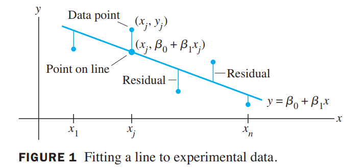
This line is also called a line of regression of $\vec{y}$ on $\vec{x}$, because any errors in the data are assumed to be only in the $y-coordinates$.
Computing the least-squares solution of $X\vec{\beta} = \vec{y}$ is equivalent to finding the $\vec{\beta}$ that determines the least-squares line in Figure 1.
The General Linear Model
Statisticians usually introduce a residual vector $\vec{\epsilon}$ defined by $\vec{\epsilon} = \vec{y} - X\vec{\beta}$, and write
$$
\vec{y} = X\vec{\beta} + \vec{\epsilon}
$$
Any equation of this form is referred to as a linear model. Once $X$ and $\vec{y}$ are determined, the goal is to minimize the length of $\vec{\epsilon}$, which amounts to finding a least-squares solution of $X\vec{\beta} = \vec{y}$.
In each case, the least-squares solution $\widehat{\vec{\beta}}$ is a solution of the normal equations:
$$
X^TX\vec{\beta} = X^T\vec{y}
$$
Least-Squares Fitting of Other Curves
The most common example is curve fitting. like
$$
y = \beta_0 + \beta_1 x + \beta_2 x^2
\tag{3}
$$
The general form is
$$
y = \beta_0 f_0(x) + \beta_1f_1(x) + \cdots + \beta_kf_k(x)
\tag{2}
$$
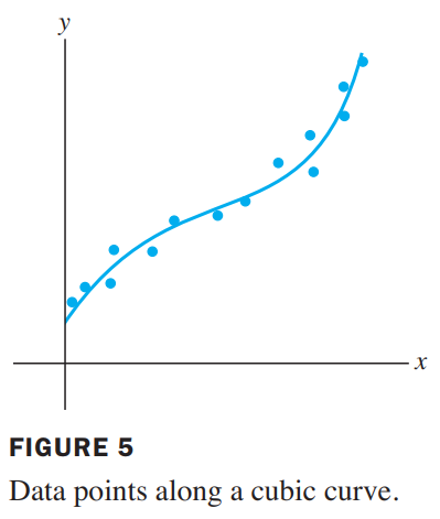
where $f_0, \cdots, f_k$ are known functions and $\beta_0, \cdots, \beta_k$ are parameters that must be determined. As we will see, equation (2) describes a linear model because it is linear in the unknown parameters.
See Figure5, it shows fitting over a cubic curve.
$$
\begin{bmatrix}
y_1\\y_2\\ \cdots \\y_n
\end{bmatrix}
=
\begin{bmatrix}
1 & x_1 & x_1^2\\
1 & x_2 & x_2^2\\
& \cdots \\
1 & x_n & x_n^2
\end{bmatrix}
\begin{bmatrix}
\beta_0\\\beta_1\\\beta_2
\end{bmatrix}
+
\begin{bmatrix}
\epsilon_1\\
\epsilon_2\\
\cdots\\
\epsilon_n\\
\end{bmatrix}
\\
\Longleftrightarrow
\\
\vec{y} = X\vec{\beta} + \vec{\epsilon}
$$
Multiple Regression
Least-squares plane.
$$
y = \beta_0 f_0(u,v) + \beta_1f_1(u,v) + \cdots + \beta_kf_k(u,v)
$$
where $f_0, \cdots, f_k$ are known functions and $\beta_0, \cdots, \beta_k$ are parameters that must be determined.
👉More about Linear Models and Least-Squares Problems in Machine Learning>>
(求最大似然函数 = 最小二乘 = 最小误差值 = 问题的最优解)
Inner Product Spaces
An inner product on a vector space $V$ is a function that, to each pair of vectors $\vec{u}$ and $\vec{v}$ in $V$ , associates a real number $\langle \vec{u}, \vec{v}\rangle$ and satisfies the following axioms, for all $\vec{u}, \vec{v}, \vec{w}$ in $V$ and all scalars $c$:
- $\langle\vec{u}, \vec{v}\rangle = \langle\vec{v}, \vec{u}\rangle$
- $\langle\vec{u + v}, \vec{w}\rangle = \langle\vec{u}, \vec{w}\rangle + \langle\vec{v}, \vec{w}\rangle$
- $\langle\vec{u}, \vec{v}\rangle = c\langle\vec{u}, \vec{v}\rangle$
- $\langle\vec{u}, \vec{u}\rangle \geq 0$ and $\langle\vec{u}, \vec{u}\rangle = 0$ if and only if $\vec{u} = \vec{0}$
A vector space with an inner product is called an inner product space.
💡For example💡:
Let $t_0, \cdots, t_n$ be distinct real numbers. For $p$ and $q$ in $P_n$, define
$$
\langle p,q\rangle = p(t_0)q(t_0) + \cdots + p(t_n)q(t_n)\\
\langle p,p\rangle = [p(t_0)]^2 + \cdots + [p(t_n)]^2
$$
Lengths, Distances, and Orthogonality
$$
||\vec{v}|| = \sqrt{\langle \vec{v}, \vec{v} \rangle}
$$
The Gram–Schmidt Process
cannot understand, to be added…
$$
$$

