Keywords: Least Squares, Bayesian Linear Regression, Evidence Approximation, Bias-Variance Decomposition, Python
This is the Chapter3 ReadingNotes from book Bishop-Pattern-Recognition-and-Machine-Learning-2006. [Code_Python]
Linear Basis Function Models
$$
y(\pmb{x}, \pmb{w}) = w_0 + w_1 x_1 + \cdots + w_Dx_D
\tag{3.1}
$$
where, $\pmb{x} = (x_1, \cdots, x_D)^T$.
$$
y(\pmb{x}, \pmb{w}) = w_0 + \sum_{j=1}^{M-1}w_j\phi_j(\pmb{x})
\tag{3.2}
$$
where, $\phi_j(\pmb{x})$ is called bisis functions, the parameter $w_0$ is called as a bias parameter.
$$
y(\pmb{x,w}) = \sum_{j=0}^{M-1}w_j\phi_j(\pmb{x}) = \pmb{w^T}\phi(\pmb{x})
\tag{3.3}
$$
where, $\phi_0{(\pmb{x})} = 1$.
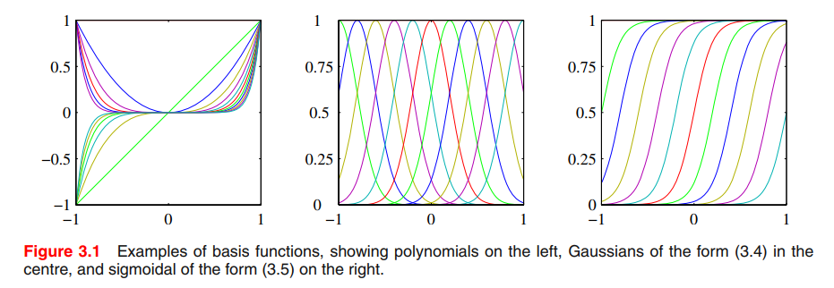
The polynomial regression considered in Chapter 1 is a particular example of this model in which there is a single input variable $x$, and the basis functions take the form of powers of $x$ so that $\phi_j(x) = x^j$.
‘Gaussian’ basis functions:
$$
\phi_j(x) = exp\lbrace -\frac{(x-\mu_j)^2}{2s^2} \rbrace
\tag{3.4}
$$
where the $\mu_j$ govern the locations of the basis functions in input space, and the parameter $s$ governs their spatial scale.
sigmoidal basis function:
$$
\phi_j(x) = \sigma(\frac{x-\mu_j}{s})
\tag{3.5}
$$
where, $\sigma(a)$ is the logistic sigmoid function defined by
$$
\sigma(a) = \frac{1}{1 + exp(-a)}
\tag{3.6}
$$
Similar function
$$
tanh(a) = 2\sigma(a)-1
$$
Maximum likelihood and least squares
Still the polynomial curve fitting problem in Chapter 1. As before, we assume that the target variable $t$ is given by a deterministic function $y(x,\pmb{w})$ with additive Gaussian noise so that
$$
t = y(x, \pmb{w}) + \epsilon
\tag{3.7}
$$
where $\epsilon$ is a zero mean Gaussian random variable with precision (inverse variance) $\beta$. Thus we can write
$$
p(t|x,\pmb{w}, \beta) = \mathcal{N}(t|y(x,\pmb{w}), \beta^{-1})
\tag{3.8}
$$
if we assume a squared loss function, then the optimal prediction, for a new value of $x$, will be given by the conditional mean of the target variable.
$$
E[t|x] = \int tp(t|x) dt = y(x,\pmb{w})
\tag{3.8}
$$
Now consider a data set of inputs $X = \lbrace x_1, \cdots, x_N \rbrace$ with corresponding target values T = $\lbrace t_1, \cdots, t_N \rbrace$. The likelihood function
$$
p(T|X,\pmb{w},\beta) = \prod_{n=1}^{N}\mathcal{N}(t_n|\pmb{w^T}\phi(x_n), \beta^{-1})
\tag{3.10}
$$
Thus,
$$
\begin{aligned}
\ln p(T|X, \pmb{w}, \beta) &= \ln p(T|\pmb{w}, \beta)\\
&=\sum_{n=1}^N\ln \mathcal{N}(t_n|\pmb{w^T}\phi(x_n),\beta^{-1})\\
&=\frac{N}{2}\ln \beta - \frac{N}{2}\ln(2\pi) - \beta E_D(\pmb{w})
\end{aligned}
\tag{3.11}
$$
where the sum-of-squares error function is defined by
$$
E_D(\pmb{w}) = \frac{1}{2} \sum_{n=1}^{N}\lbrace t_n - \pmb{w^T}\phi(x_n)\rbrace^2
\tag{3.12}
$$
The gradient of the log likelihood function (3.11) takes the form
$$
\nabla \ln p(T|\pmb{w},\beta) = \sum_{n=1}^N \lbrace t_n - \pmb{w^T}\phi(x_n)\rbrace \phi(x_n)^T
\tag{3.13}
$$
Setting this gradient to zero gives
$$
0 = \sum_{n=1}^{N} t_n \phi(x_n)^T - \pmb{w^T}(\sum_{n=1}^{N}\phi(x_n)\phi(x_n)^T)
\tag{3.14}
$$
Solving for $\pmb{w}$ we obtain
$$
\pmb{w}_{ML} = (\Phi^T\Phi)^{-1}\Phi^T T
\tag{3.15}
$$
which are known as the normal equations for the least squares problem. Here $\Phi$ is an $N \times M$ matrix, called the design matrix, whose elements are given by $\Phi_{nj} = \phi_j(x_n)$, so that
$$
\Phi =
\begin{bmatrix}
\phi_0(x_1) & \phi_1(x_1) & \cdots & \phi_{M-1}(x_1) \\
\phi_0(x_2) & \phi_1(x_2) & \cdots & \phi_{M-1}(x_2) \\
\vdots & \vdots & \ddots & \vdots\\
\phi_0(x_N) & \phi_1(x_N) & \cdots & \phi_{M-1}(x_N)
\end{bmatrix}
$$
👉Least Squares in Numerical Analysis >>
Moore-Penrose pseudo-inverse of the matrix $\Phi$ is:
$$
\Phi^\dagger = (\Phi^T\Phi)^{-1}\Phi^T
$$
Now back to $w_0$, the bias parameter. the error function (3.12)
$$
\begin{aligned}
E_D(\pmb{w}) &= \frac{1}{2} \sum_{n=1}^{N}\lbrace t_n - \pmb{w^T}\phi(x_n)\rbrace^2 \\
&= \frac{1}{2} \sum_{n=1}^{N}\lbrace t_n - w_0 -\sum_{j=1}^{M-1} w_j\phi_j(x_n)\rbrace^2
\end{aligned}
\tag{3.18}
$$
Setting the derivative with respect to $w_0$ equal to zero, and solving for $w_0$, we obtain
$$
w_0 = \bar{t} - \sum_{j=1}^{M-1}w_j\bar{\phi_j}
\tag{3.19}
$$
where,
$$
\bar{t} = \frac{1}{N}\sum_{n=1}^{N} t_n\\
\bar{\phi_j} = \frac{1}{N}\sum_{n=1}^{N}\phi_j(x_n)
\tag{3.20}
$$
Thus the bias $w_0$ compensates for the difference between the averages (over the training set) of the target values and the weighted sum of the averages of the basis function values.
We can also maximize the log likelihood function (3.11) with respect to the noise precision parameter $\beta$, giving
$$
\frac{1}{\beta_{ML}} = \frac{1}{N} \sum_{n=1}^{N} \lbrace t_n - \pmb{w_{ML}^T} \phi(x_n)\rbrace^2
\tag{3.21}
$$
so we see that the inverse of the noise precision is given by the residual variance of the target values around the regression function.
Geometry of least squares

Note that $\psi_j$ corresponds to the $j^{th}$ column of $\Phi$, whereas $\phi(x_n)$ corresponds to the $n^{th}$ row of $\Phi$.
We define $y$ to be an $N$-dimensional vector whose $n^{th}$ element is given by $y(x_n,\pmb{w})$, where $n = 1, . . . , N$.
Sequential learning
Batch techniques, such as the maximum likelihood solution (3.15), which involve processing the entire training set in one go, can be computationally costly for large data sets.
it may be worthwhile to use sequential algorithms, also known as on-line algorithms, in which the data points are considered one at a time, and the model parameters updated after each such presentation.
We can obtain a sequential learning algorithm by applying the technique of stochastic gradient descent(随机梯度下降), also known as sequential gradient descent, as follows.
If the error function comprises a sum over data points $E = \sum_n E_n$, then after presentation of pattern $n$, the stochastic gradient descent algorithm updates the parameter vector $\pmb{w}$ using
$$
\pmb{w}^{\tau + 1} = \pmb{w}^\tau - \eta \nabla E_n
\tag{3.22}
$$
where, $\tau$ denotes the iteration number, and $\eta$ is a learning rate parameter.
For the case of the sum-of-squares error function (3.12), this gives
$$
\pmb{w}^{\tau + 1} = \pmb{w}^\tau + \eta (t_n - \pmb{w}^{(\tau)T} \phi_n)\phi_n
\tag{3.23}
$$
where $\phi_n = \phi(x_n)$.
This is known as least-mean-squares or the LMS algorithm.
Regularized least squares
To control over-fitting, we introduced a regularization term to an error function:
$$
E_D(\pmb{w}) + \lambda E_W(\pmb{w}) =
\frac{1}{2}\sum_{n=1}^{N}\lbrace t_n - \pmb{w^T}\phi(x_n)\rbrace^2 + \frac{\lambda}{2}\pmb{w^T}\pmb{w}
\tag{3.27}
$$
This particular choice of regularizer is known in the machine learning literature as weight decay because in sequential learning algorithms, it encourages weight values to decay towards zero, unless supported by the data.
A more general regularizer is sometimes used, for which the regularized error takes the form
$$
\frac{1}{2}\sum_{n=1}^{N}\lbrace t_n - \pmb{w^T}\phi(x_n)\rbrace^2 + \frac{\lambda}{2}\sum_{j=1}^{M}|w_j|^q
\tag{3.29}
$$
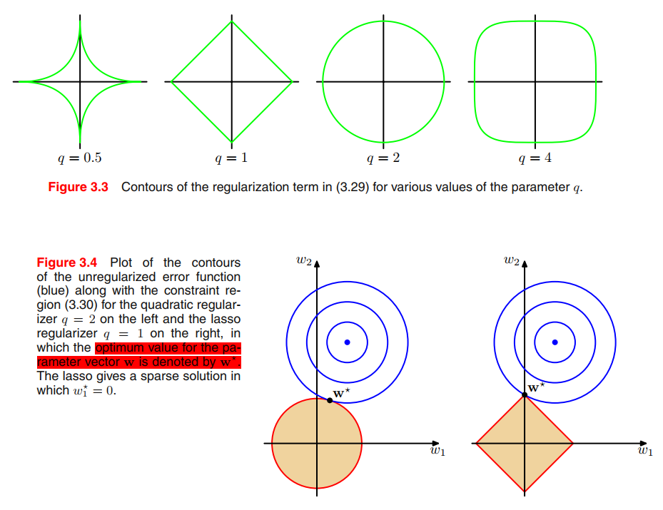
where $q = 2$ corresponds to the quadratic regularizer (3.27). Figure 3.3 shows contours of the regularization function for different values of $q$.
minimizing (3.29) is equivalent to minimizing the unregularized sum-of-squares error (3.12) subject to the constraint
$$
\sum_{j=1}^{M}|w_j|^q \leq \eta
\tag{3.30}
$$
for an appropriate value of the parameter $\eta$, where the two approaches can be related using 👉Lagrange multipliers.
Multiple outputs
$$
\pmb{y(x,w)} = \pmb{W^T} \phi(\pmb{x})
\tag{3.31}
$$
Here, $\pmb{t}$ or $\pmb{y(x,w)}$ is not a single target variable, but a $K$-dimensional vector. $\pmb{W}$ is an $M \times K$ matrix of parameters. $\phi(\pmb{x})$ is an $M$-dimensional column vector with elements $\phi_j(x)$, $\phi_0(x) = 1$ as before.
Suppose we take the conditional distribution of the target vector to be an isotropic Gaussian of the form
$$
p(\pmb{t}|\pmb{x}, \pmb{W}, \beta) = \mathcal{N}(\pmb{t}|\pmb{W^T\phi(x)}, \beta^{-1}I)
\tag{3.32}
$$
If we have a set of observations $\pmb{t_1}, \cdots, \pmb{t_N}$, we can combine these into a matrix $\pmb{T}$ of size $N \times K$ such that the $n^{th}$ row is given by $\pmb{t^T_n}$.
The Bias-Variance Decomposition
As we have seen in earlier chapters, the phenomenon of over-fitting is really an unfortunate property of maximum likelihood and does not arise when we marginalize over parameters in a Bayesian setting.
Here we generate $100$ data sets, each containing $N = 25$ data points, independently from the sinusoidal curve $h(x) = \sin (2\pi x)$. The data sets are indexed by $l = 1, \cdots, L$, where $L = 100$, and for each data set $D^{(l)}$ we fit a model with 24 Gaussian basis functions by minimizing the regularized error function (3.27) to give a prediction function $y^{(l)}(x)$ as shown in Figure 3.5.
$$
E_D(\pmb{w}) + \lambda E_W(\pmb{w}) =
\frac{1}{2}\sum_{n=1}^{N}\lbrace t_n - \pmb{w^T}\phi(x_n)\rbrace^2 + \frac{\lambda}{2}\pmb{w^T}\pmb{w}
\tag{3.27}
$$
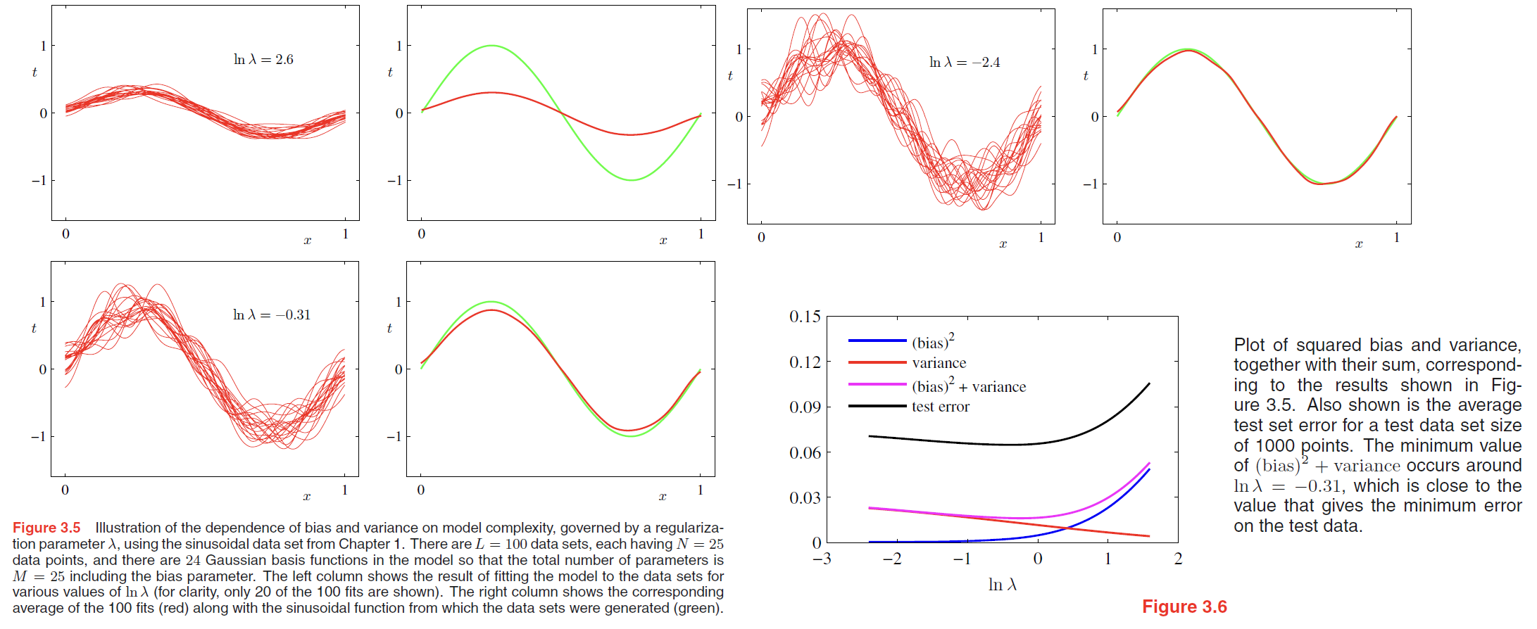
The top row corresponds to a large value of the regularization coefficient $\lambda$ that gives low variance (because the red curves in the left plot look similar) but high bias (because the two curves in the right plot are very different).
Conversely on the bottom row, for which $\lambda$ is small, there is large variance (shown by the high variability between the red curves in the left plot) but low bias (shown by the good fit between the average model fit and the original sinusoidal function).
Now we consider a frequentist viewpoint of the model complexity issue, known as the bias-variance trade-off.
For regression problem, we considered various loss functions each of which leads to a corresponding optimal prediction once we are given the conditional distribution(called predictive distribution in Chapter 1) $p(t|x)$. A popular choice is the squared loss function, for which the optimal prediction is given by the conditional expectation, which we denote by $h(x)$ and which is given by
$$
h(x) = E[t|x] = \int t p(t|x) dt
\tag{3.36}
$$
the expected squared loss can be written in the form
$$
E[L] = \int \lbrace y(x) - h(x)\rbrace ^2 p(x) dx + \int \lbrace h(x) - t\rbrace^2 p(x,t) dx dt
\tag{3.37}
$$
For any given data set $D$, we can run our learning algorithm and obtain a prediction function $y(x;D)$.
Consider the integrand of the first term in (3.37), which for a particular data set $D$ takes the form
$$
\lbrace y(x; D) - h(x)\rbrace^2
\tag{3.38}
$$
We now take the expectation of this expression with respect to $D$ and note that the final term will vanish, giving
$$
E_D[\lbrace y(x;D) - h(x)\rbrace^2] = \underbrace{\lbrace E_D[y(x;D)] - h(x) \rbrace ^2}_{bias^2} +
$$
$$
\underbrace{E_D[\lbrace y(x;D) - E_D[y(x;D)] \rbrace^2]}_{variance}
\tag{3.40}
$$
So far, we have considered a single input value $x$. If we substitute this expansion back into (3.37)(代入展开式到3.37), we obtain the following decomposition of the expected squared loss(平方期望损失)
$$
expected \space loss = (bias)^2 + variance + noise
\tag{3.41}
$$
where,
$$
(bias)^2 = \int \lbrace E_D{y(x;D)} - h(x)\rbrace ^2 p(x) dx
\tag{3.42}
$$
$$
variance = \int E_D[\lbrace y(x;D - E_D[y(x;D)]\rbrace^2)] p(x) dx
\tag{3.43}
$$
$$
noise = \int \lbrace h(x) - t\rbrace^2 p(x,t) dx dt
$$
The model with the optimal predictive capability is the one that leads to the best balance between bias and variance.
Back to the fitting problem, the average prediction is estimated from
$$
\bar{y}(x) = \frac{1}{L} \sum_{l=1}^L y^{(l)} (x)
\tag{3.45}
$$
and the integrated squared bias and integrated variance are then given by
$$
(bias)^2 = \frac{1}{N} \sum_{n=1}^{N} \lbrace \bar{y}(x_n) - h(x_n)\rbrace^2
\tag{3.46}
$$
$$
variance = \frac{1}{N} \sum_{n=1}^{N} \frac{1}{L} \sum_{l=1}^L \lbrace y^{(l)}(x_n) - \bar y (x_n) \rbrace^2
\tag{3.47}
$$
Although the bias-variance decomposition may provide some interesting insights into the model complexity issue from a frequentist perspective, it is of limited practical value, because the bias-variance decomposition is based on averages with respect to ensembles of data sets, whereas in practice we have only the single observed data set.
If we had a large number of independent training sets of a given size, we would be better off combining them into a single large training set, which of course would reduce the level of over-fitting for a given model complexity.
Given these limitations, we turn in the next section to a Bayesian treatment of linear basis function models, which not only provides powerful insights into the issues of over-fitting but which also leads to practical techniques for addressing the question model complexity.
Bayesian Linear Regression
We now turn to a Bayesian treatment of linear regression, which will avoid the over-fitting problem of maximum likelihood, and which will also lead to automatic methods of determining model complexity using the training data alone.
Parameter distribution
we shall treat the noise precision parameter $β$ as a known constant, thus, equation (3.10) becomes
$$
p(T|X,\pmb{w},\beta) \Leftrightarrow p(T|\pmb{w})\\
= \prod_{n=1}^{N}\mathcal{N}(t_n|\pmb{w^T}\phi(x_n), \beta^{-1})
$$
this function is a exponential of a quadratic function of $\pmb{w}$. The corresponding conjugate prior is therefore given by a Gaussian distribution of the form
$$
p(\pmb{w}) = \mathcal{N}(\pmb{w}|\pmb{m_0},\pmb{S_0})
\tag{3.48}
$$
having mean $\pmb{m_0}$ and covariance $\pmb{S_0}$.
Next we compute the posterior distribution, which is proportional to the product of the likelihood function and the prior.
$$
p(\pmb{w}|T) \propto p(T|\pmb{w}) p(\pmb{w})
$$
thus,
$$
p(\pmb{w}|T) = \mathcal{N}(\pmb{w}|\pmb{m_N},\pmb{S_N})
\tag{3.49}
$$
where,
$$
\pmb{m_N }= \pmb{S_N}(\pmb{S_0^{-1}m_0} + \beta \pmb{\Phi^TT})
\tag{3.50}
$$
$$
\pmb{S_N^{-1}} = \pmb{S_0^{-1}} + \beta \pmb{\Phi^T\Phi}
\tag{3.51}
$$
For simplicity, we consider a zero-mean isotropic Gaussian governed by a single precision parameter $\alpha$ so that
$$
p(\pmb{w}|\alpha) = \mathcal{N}(\pmb{w}|\pmb{0}, \alpha^{-1}\pmb{I})
\tag{3.52}
$$
and the corresponding posterior distribution over $\pmb{w}$ is then given by (3.49) with
$$
\pmb{m_N} = \beta \pmb{S_N}\pmb{\Phi^T}T
\tag{3.53}
$$
$$
\pmb{S_N^{-1}} = \alpha \pmb{I} + \beta \pmb{\Phi^T\Phi}
\tag{3.54}
$$
💡For example💡:
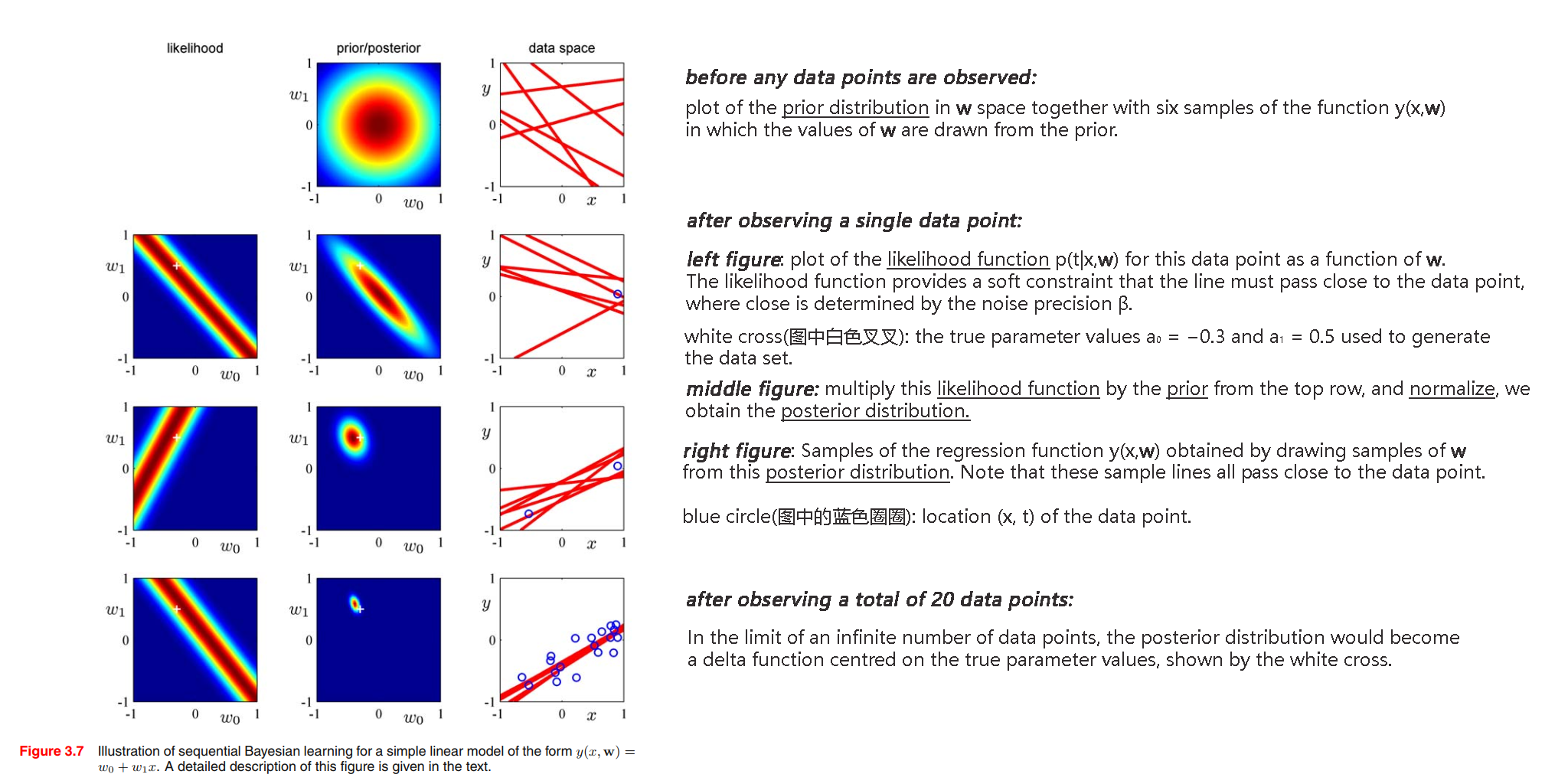
We can illustrate Bayesian learning in a linear basis function model, as well as the sequential update of a posterior distribution, using a simple example involving straight-line fitting.
$$
y(x,\pmb{w}) = w_0 + w_1x
$$
We generate points data by function $f(x,\pmb{a}) = a_0 + a_1 x =-0.3 + 0.5 x$, using $x_n$ from uniform distribution $\mathcal{U}(x | -1, 1)$, then evaluating $f(x_n, \pmb{a})$, and finally adding Gaussian noise with standard deviation of $0.2$ to obtain the target values $t_n$.
Our goal is to recover the values of $a_0$ and $a_1$ from such data.
Solution:
Predictive distribution
In practice, we are not usually interested in the value of $\pmb{w}$ itself but rather in making predictions of $t$ for new values of $x$. This requires that we evaluate the predictive distribution defined by
$$
p(t|T,\alpha, \beta) = \int p(t|\pmb{w}, \beta) p(w|T,\alpha, \beta) d\pmb{w}
\tag{3.57}
$$
The conditional distribution $p(t|x, \pmb{w}, \beta)$ of the target variable is given by (3.8), and the posterior weight distribution is given by (3.49).
$$
p(t|x,T,\alpha, \beta) = \mathcal{N}(t|\pmb{m_N^T\phi(x)}, \sigma^2_N(x))
\tag{3.58}
$$
where the variance $\sigma^2_N(x)$ of the predictive distribution is given by
$$
\sigma^2_N(x) = \frac{1}{\beta} + \phi(x)^T\pmb{S_N}\phi(x)
\tag{3.59}
$$
The first term in (3.59) represents the noise on the data whereas the second term reflects the uncertainty associated with the parameters $\pmb{w}$. Because the noise process and the distribution of $\pmb{w}$ are independent Gaussians, their variances are additive.
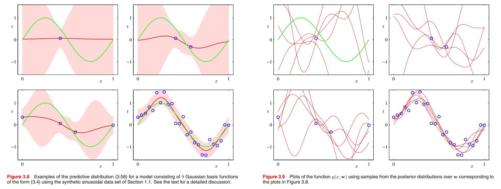
we fit a model comprising a linear combination of Gaussian basis functions to data sets of various sizes and then look at the corresponding posterior distributions. Here the green curves correspond to the function $\sin(2\pi x)$ from which the data points were generated (with the addition of Gaussian noise). Data sets of size $N = 1, N = 2, N = 4$, and $N = 25$ are shown in the four plots by the blue circles. For each plot, the red curve shows the mean of the corresponding Gaussian predictive distribution, and the red shaded region spans one standard deviation either side of the mean. Note that the predictive uncertainty depends on $x$ and is smallest in the neighbourhood of the data points. Also note that the level of uncertainty decreases as more data points are observed.
The plots in Figure 3.8 only show the point-wise predictive variance as a function of $x$. In order to gain insight into the covariance between the predictions at different values of $x$, we can draw samples from the posterior distribution over $\pmb{w}$, and then plot the corresponding functions $y(x,\pmb{w})$, as shown in Figure 3.9.
If we used localized basis functions such as Gaussians, then in regions away from the basis function centres, the contribution from the second term in the predictive variance (3.59) will go to zero, leaving only the noise contribution $\frac{1}{\beta}$.
Thus, the model becomes very confident in its predictions when extrapolating outside the region occupied by the basis functions, which is generally an undesirable behaviour. This problem can be avoided by adopting an alternative Bayesian approach to regression known as a Gaussian process.
Equivalent kernel
If we substitute (3.53) into the expression (3.3), we see that the predictive mean can be written in the form
$$
\pmb{m_N} = \beta \pmb{S_N}\pmb{\Phi^T}T
\tag{3.53}
$$
$$
y(\pmb{x,w}) = \sum_{j=0}^{M-1}w_j\phi_j(\pmb{x}) = \pmb{w^T}\phi(\pmb{x})
\tag{3.3}
$$
$$
\begin{aligned}
y(x, m_N) &= m_N^T \phi(x)\\
&= \beta \phi(x)^TS_N \Phi^T T \\
&= \sum_{n=1}^N \beta \phi(x)^T S_N \phi(x_n) t_n
\end{aligned}
\tag{3.60}
$$
where $S_N$ is defined by (3.51).
$$
\pmb{S_N^{-1}} = \pmb{S_0^{-1}} + \beta \pmb{\Phi^T\Phi}
\tag{3.51}
$$
Thus the mean of the predictive distribution at a point $x$ is given by a linear combination of the training set target variables $t_n$, so that we can write
$$
y(x, m_N) = \sum_{n=1}^N k(x,x_n) t_n
\tag{3.61}
$$
where the function
$$
k(x,x’) = \beta \phi(x)^T S_N \phi(x’)
\tag{3.62}
$$
is known as the smoother matrix or the equivalent kernel.
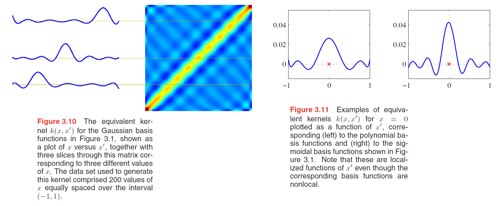
The equivalent kernel is illustrated for the case of Gaussian basis functions in Figure 3.10 in which the kernel functions $k(x, x’)$ have been plotted as a function of $x’$ for three different values of $x$.
We see that they are localized around $x$, and so the mean of the predictive distribution at $x$, given by $y(x,m_N)$, is obtained by forming a weighted combination of the target values in which data points close to $x$ are given higher weight than points further removed from $x$.
Further insight into the role of the equivalent kernel can be obtained by considering the covariance between $y(x)$ and $y(x’)$, which is given by
$$
\begin{aligned}
cov[y(x), y(x’)] &= cov[phi(x)^T w, w^T phi(x’)] \\
&= \phi(x)^T S_N \phi(x’) \\
&= \beta^{-1}k(x,x’)
\end{aligned}
\tag{3.63}
$$
From the form of the equivalent kernel, we see that the predictive mean at nearby points will be highly correlated, whereas for more distant pairs of points the correlation will be smaller.
The formulation of linear regression in terms of a kernel function suggests an alternative approach to regression as follows. Instead of introducing a set of basis functions, which implicitly determines an equivalent kernel, we can instead define a localized kernel directly and use this to make predictions for new input vectors $x$, given the observed training set. This leads to a practical framework for regression (and classification) called Gaussian processes.
Bayesian Model Comparison
As we shall see, the over-fitting associated with maximum likelihood can be avoided by marginalizing (summing or integrating) over the model parameters instead of making point estimates of their values.
Suppose we wish to compare a set of $L$ models $\lbrace M_i\rbrace$, where $i = 1, \cdots, L$. Here a model refers to a probability distribution
over the observed data $D$. We shall suppose that the data is generated from one of these models but we are uncertain which one.
Our uncertainty is expressed through a prior probability distribution $p(M_i)$. Given a training set $D$, we then wish to evaluate the posterior distribution
$$
p(M_i | D) \propto p(M_i) \underbrace{p(D|M_i)}_{model-evidence}
\tag{3.66}
$$
model-evidence expresses the preference shown by the data for different models, it is also called the marginal likelihood because it can be viewed as a likelihood function over the space of models, in which the parameters have been marginalized out.
The ratio of model evidences $p(D|M_i)/p(D|M_j)$ for two models is known as a Bayes factor.
The predictive distribution is given by,
$$
p(t|x, D) = \sum_{i=1}^L p(t|x, M_i, D) p(M_i| D)
\tag{3.67}
$$
This is an example of a mixture distribution in which the overall predictive distribution is obtained by averaging the predictive distributions $p(t|x,M_i,D)$ of individual models, weighted by the posterior probabilities $p(M_i|D)$ of those models.
For a model governed by a set of parameters $\pmb{w}$, the model evidence is given, from the sum and product rules of probability, by
$$
\underbrace{p(D|M_i)}_{model-evidence} = \int p(D|\pmb{w}, M_i) p(\pmb{w}|M_i) d\pmb{w}
\tag{3.68}
$$
From a sampling perspective, the marginal likelihood can be viewed as the probability of generating the data set $D$ from a model whose parameters are sampled at random from the prior.
It is also interesting to note that the evidence is precisely the normalizing term that appears in the denominator in Bayes’ theorem when evaluating the posterior distribution over parameters because
$$
p(\pmb{w} | D, M_i) = \frac{p(D|\pmb{w}, M_i) p(\pmb{w} | M_i)}{p(D | M_i)}
\tag{3.69}
$$
Consider first the case of a model having a single parameter $w$. The posterior distribution over parameters is proportional to
$p(D|w)p(w)$, where we omit the dependence on the model $M_i$ to keep the notation uncluttered.
If we assume that the posterior distribution is sharply peaked around the most probable value $w_{MAP}$, with width $\Delta w_{posterior}$, then we can approximate the integral by the value of the integrand at its maximum times the width of the peak.
If we further assume that the prior is flat with width $\Delta w_{prior}$ so that $p(w) = 1/\Delta w_{prior}$, then we have
$$
p(D) = \int p(D|w) p(w) dw \simeq p(D|w_{MAP}) \frac{\Delta w_{posterior}}{\Delta w_{prior}}
\tag{3.70}
$$
so taking logs we obtain
$$
\ln p(D) \simeq \ln p(D|w_{MAP}) + \ln \frac{\Delta w_{posterior}}{\Delta w_{prior}}
\tag{3.71}
$$

The Evidence Approximation
Here we discuss an approximation in which we set the hyperparameters to specific values determined by maximizing the marginal likelihood function obtained by first integrating over the parameters $\pmb{w}$. This framework is known in the statistics literature as empirical Bayes.
If we introduce hyperpriors over $\alpha$ and $\beta$, the predictive distribution is obtained by marginalizing over $\pmb{w}$, $\alpha$ and $\beta$ so that
$$
p(t|T) = \int \int \int p(t | \pmb{w}, \beta) p(\pmb{w} | T, \alpha, \beta) p(\alpha, \beta | T) d\pmb{w} d\alpha d\beta
\tag{3.74}
$$
where $p(t | \pmb{w}, \beta)$ is given by
$$
p(t|x,\pmb{w}, \beta) = \mathcal{N}(t|y(x,\pmb{w}), \beta^{-1})
\tag{3.8}
$$
$p(\pmb{w} | T, \alpha, \beta)$ is given by
$$
p(\pmb{w}|T) = \mathcal{N}(\pmb{w}|\pmb{m_N},\pmb{S_N})
\tag{3.49}
$$
If the posterior distribution $p(\alpha, \beta | T)$ is sharply peaked around values $\hat{\alpha}$ and $\hat{\beta}$, then the predictive distribution is obtained simply by marginalizing over $\pmb{w}$ in which $\alpha$ and $\beta$ are fixed to the values $\hat{\alpha}$ and $\hat{\beta}$, so that
$$
p(t|T) \simeq p(t|T,\hat{\alpha}, \hat{\beta}) = \int p(t | \pmb{w}, \hat{\beta}) p(\pmb{w} | T, \hat{\alpha}, \hat{\beta}) d\pmb{w}
\tag{3.75}
$$
From Bayes’ theorem, the posterior distribution for $\alpha$ and $\beta$ is given by
$$
p(\alpha, \beta | T) \propto p(T | \alpha, \beta) p(\alpha, \beta)
\tag{3.76}
$$
If the prior is relatively flat, then in the evidence framework the values of $\hat{\alpha}$ and $\hat{\beta}$ are obtained by maximizing the marginal likelihood function $p(T | \alpha, \beta)$.

