Keywords: Contrastive Learning, SMPL, SMAL, 3D-CoreNet, 2023
MAPConNet: Self-supervised 3D Pose Transfer with Mesh and Point Contrastive Learning_ICCV_2023
Jiaze Sun1* Zhixiang Chen2 Tae-Kyun Kim1,3
1 Imperial College London
2 University of Sheffield
3 Korea Advanced Institute of Science and Technology
https://github.com/justin941208/MAPConNet
Challenge
One of the main challenges of 3D pose transfer is that current methods still put certain requirements on their training data making it difficult to collect and expensive to annotate.
Innovation
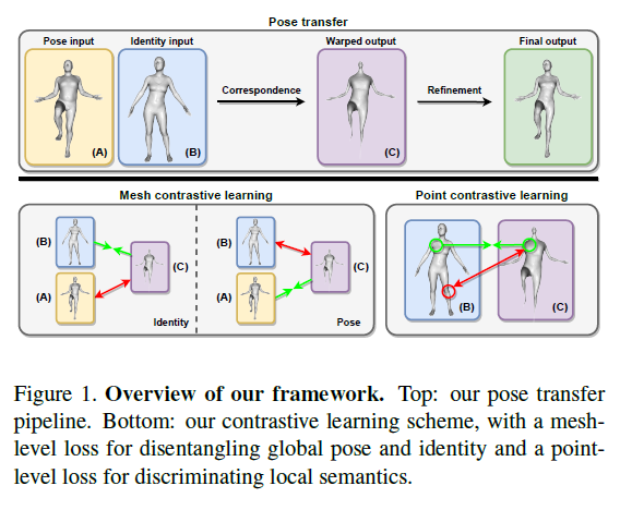
To prevent the network from exploiting shortcuts in unsupervised learning that circumvent the desired objective, we introduce disentangled latent pose and identity representations.
To strengthen the disentanglement and guide the learning process more effectively, we propose mesh-level contrastive learning to force the model’s intermediate output to have matching latent identity and pose representations with the respective inputs.
To further improve the quality of the model’s intermediate output as well as the correspondence module, we also propose point-level contrastive learning, which enforces similarity between representations of corresponding points and dissimilarity between non-corresponding ones.
Workflow
3D-CoreNet
It has two modules: correspondence and refinement. The training of 3D-CoreNet is supervised, given the model output $\hat{\pmb{x}}^{B1}$ and the ground truth output $\pmb{x}^{B1}$, it minimises the reconstruction loss
$$
L_{rec}(\hat{\pmb{x}}^{B1}; \pmb{x}^{B1}) = \frac{1}{3N_{id}} ||\hat{\pmb{x}}^{B1} - \pmb{x}^{B1}||_F^2
\tag{1}
$$
$$
L_{edge}(\hat{\pmb{x}}^{B1}; \pmb{x}^{B2}) = \frac{1}{\xi} \sum_{(j,k) \in \xi} |\frac{||\hat{\pmb{x_j}}^{B1} - \hat{\pmb{x_k}}^{B1}||_2}{||\pmb{x_j}^{B2} - \pmb{x_k}^{B2}||_2} - 1|
\tag{2}
$$
where $\xi$ is the set of all index pairs representing vertices that are connected by an edge, and $\hat{\pmb{x_j}}^{B1}, \pmb{x_j}^{B2}$ are the coordinates of the $j$-th (similarly, $k$-th) vertices of $\hat{\pmb{x}}^{B1}$ and $\pmb{x}^{B2}$ respectively.
Finally, the overall supervised loss is given by
$$
L_s = \lambda_{rec} L_{rec}(\hat{\pmb{x}}^{B1}; \pmb{x}^{B1}) + \lambda_{edge}L_{edge}(\hat{\pmb{x}}^{B1}; \pmb{x}^{B2})
\tag{3}
$$
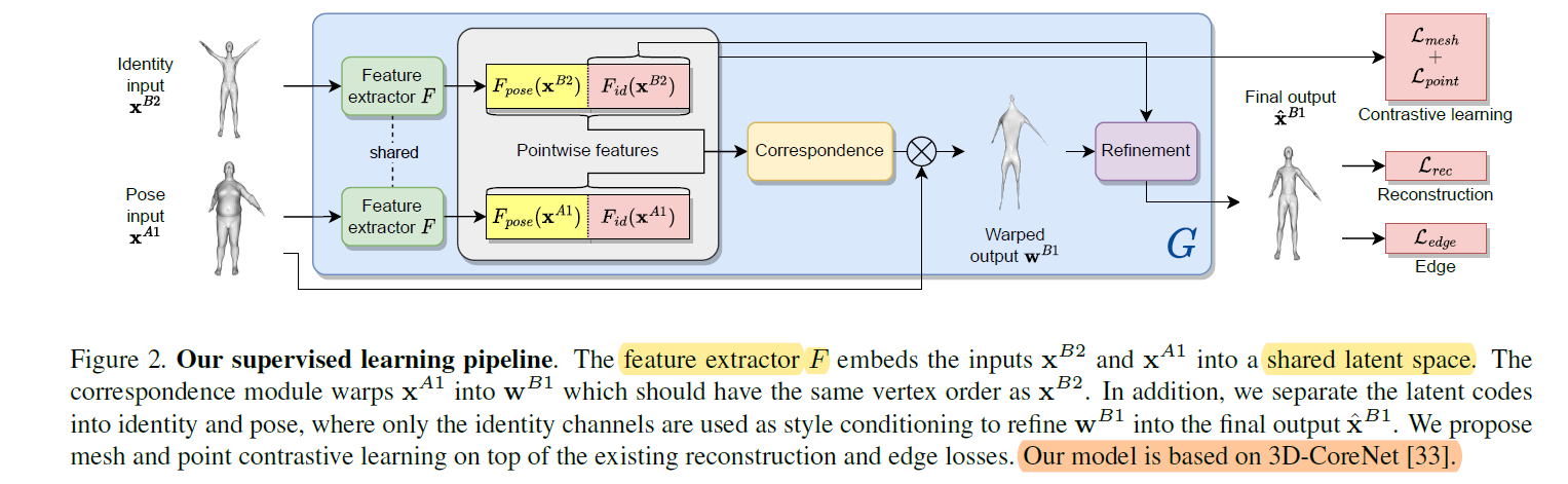
Correspondence Module
The correspondence module produces an intermediate “warped” output $\pmb{w}^{B1} \in R^{N_{id} \times 3}$ inheriting the pose from $\pmb{x}^{A1}$ but the vertex order of $\pmb{x}^{B2}$,
$$
\pmb{w}^{B1} = \pmb{T}\pmb{x}^{A1}
$$
where
$$
\pmb{T} \in R_{+}^{N_{id} \times N_{pose}}
$$
is an optimal transport (OT) matrix learned based on the latent features of both inputs.
Refinement Module
The refinement module then uses the features of the identity input $\pmb{x}^{B2}$ as style condition for the warped output $\pmb{w}^{B1}$, refining it through elastic instance normalisation and producing the final output $\hat{\pmb{x}}^{B1}$.
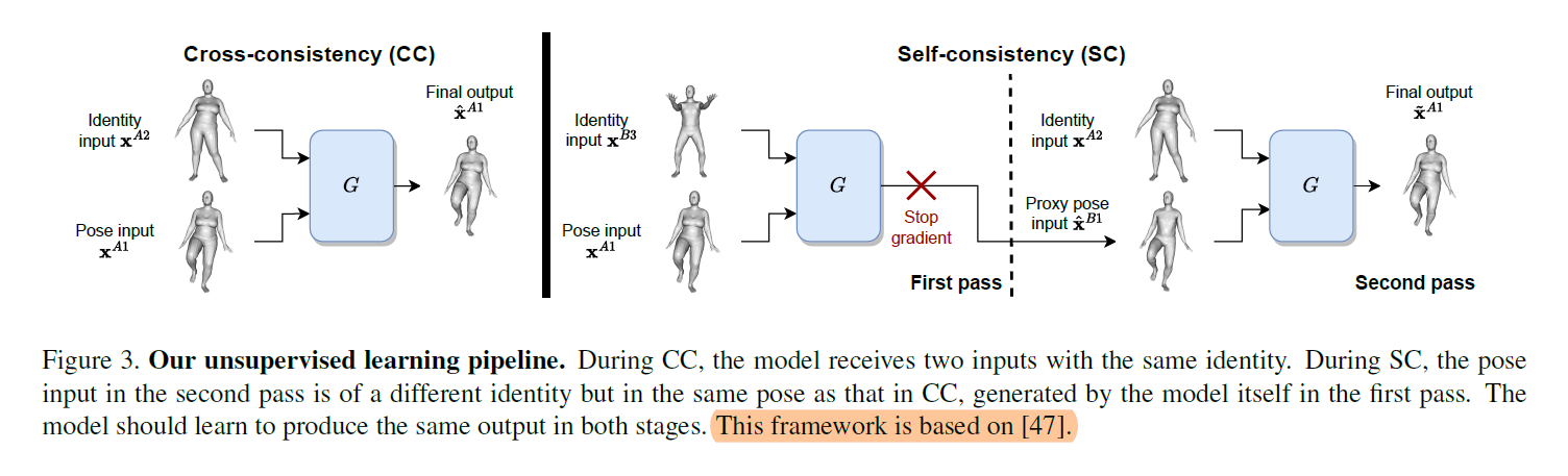
Unsupervised Pose Transfer
we present our unsupervised pipeline with the self- and cross-consistency losses by [47]. (a) when both inputs share a common identity, and (b) when the pose input in (a) is replaced by a different identity with the same pose. Task (a) is called “cross-consistency” and is readily available from the dataset. The pose input in task (b) is unavailable but can be generated by the network itself, i.e. “self-consistency”.
The overall unsupervised loss is given by
$$
L_{us} = L_{cc} + L{sc}
\tag{6}
$$
Cross-Consistency
the network should reconstruct $\pmb{x}^{A1}$, through $\hat{\pmb{x}}^{A1} = G(\pmb{x}^{A1}, \pmb{x}^{A2})$ (Figure 3, left). This is enforced via
$$
L_{cc} = \lambda_{rec} L_{rec}(\hat{\pmb{x}}^{A1}; \pmb{x}^{A1}) + \lambda_{edge}(\hat{\pmb{x}}^{A1}; \pmb{x}^{A2})
\tag{4}
$$
Self-Consistency
As mentioned previously, the model should reconstruct the same output as that in CC when its pose input is replaced by a different identity with the same pose – which is usually not available from the training data.
In the first pass, given pose input $\pmb{x}^{A1}$ and identity input $\pmb{x}^{B3}$, the network generates a proxy $\hat{\pmb{x}}^{B1} = G(\pmb{x}^{A1}, \pmb{x}^{B3})$.
In the second pass, reconstruct the initial pose input $\widetilde{\pmb{x}}^{A1} = G(SG(\hat{\pmb{x}}^{B1}), \pmb{x}^{A2})$. where $SG$ stops the gradient from passing through.
The purpose of $SG$ is to prevent the model from exploiting shortcuts such as using the input $\pmb{x}^{A1}$ from the first pass to directly reconstruct the output in the second pass.
The SC loss is
$$
L_{sc} = \lambda_{rec} L_{rec}(\widetilde{\pmb{x}}^{A1}; \pmb{x}^{A1}) + \lambda_{edge}(\widetilde{\pmb{x}}^{A1}; \pmb{x}^{A2})
\tag{5}
$$
Latent disentanglement of pose and identity
we disentangle the latents into pose and identity channels. This allows us to impose direct constraints on the meaning of these channels to improve the accuracy of the model output.
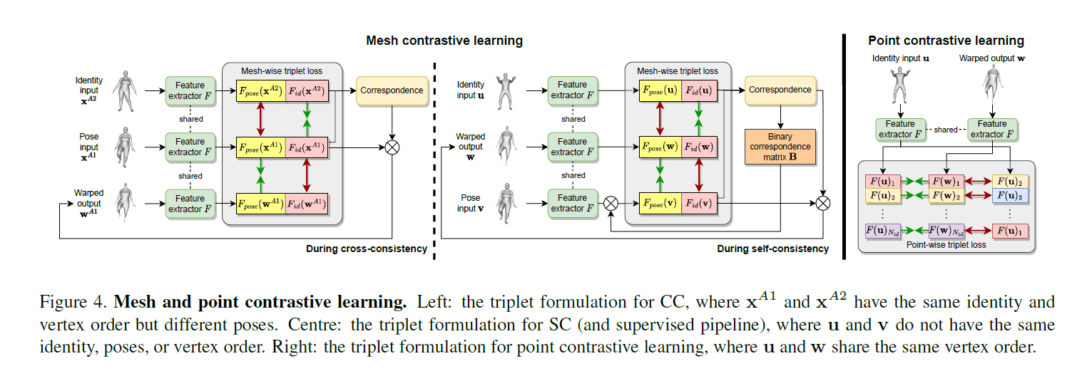
Mesh Contrastive Learning
As we cannot compare pose and identity directly in the mesh space, we take a self supervised approach by feeding meshes through the feature extractor $F$ and imposing the triplet loss [32] on the latent representations (see Figure 4). Specifically, given an anchor latent $\pmb{a}$, a positive latent $\pmb{p}$, and a negative latent $\pmb{n}$ which are all in $R^{N \times D}$, our mesh triplet loss is given by
$$
l(\pmb{a,p,n}) = (m + \frac{1}{N} \sum_{j=1}^N d(\pmb{a_j, p_j, n_j}))^{+}
\tag{7}
$$
where
$$
(\cdot)^{+} = max(0, \cdot)
$$
$m$ is the margin,
$$
d(\pmb{a_j, p_j, n_j}) = ||a_j, p_j||_2 - ||a_j, n_j||_2
\tag{8}
$$
Contrastive learning in CC
By intuition, the pose representation of $\pmb{x}^{A1}$ should be closer to that of $\pmb{w}^{A1}$ than $\pmb{x}^{A2}$, the identity representation of $\pmb{x}^{A1}$ should be closer to that of $\pmb{x}^{A2}$ than $\pmb{w}^{A1}$ as $\pmb{w}^{A1}$ should generally avoid inheriting the identity representation from the pose input. Hence,
$$
L_{mesh}^{cc} = l(F_{pose}(\pmb{x}^{A1}), F_{pose}(\pmb{w}^{A1}), F_{pose}(\pmb{x}^{A2})) + l(F_{id}(\pmb{x}^{A1}), F_{id}(\pmb{x}^{A2}), F_{id}(\pmb{w}^{A1}))
\tag{9}
$$
Contrastive learning in SC
However, unlike CC, the vertex orders of $\pmb{u}$ and $\pmb{v}$ in SC are not aligned. As a result, equations 7 and 8 cannot be applied directly as they only compare distances between aligned vertices.
We again take a self-supervised approach to “reorder” the feature of $\pmb{v}$ by utilising the OT matrix $\pmb{T}$.
As the cost matrix for OT is based on the pairwise similarities between point features of $\pmb{u}$ and $\pmb{v}$, most entries in $\pmb{T}$ are made close to zero except for a small portion which are more likely to be corresponding points. Therefore, we use the following binary version of $\pmb{T}$ to select vertices from $\pmb{v}$
$$
\pmb{B_{jk}} = I \lbrace \pmb{T_{jk}} = \underbrace{max}_{l} \pmb{T_{jl}} \rbrace
\tag{10}
$$
In other words, each row of $\pmb{B} \in \lbrace 0, 1 \rbrace ^{N_{id} \times N_{pose}}$ is a binary vector marking the location of the maximum value in the corresponding row of $\pmb{T}$. We further constrain the rows of $\pmb{B}$ to be one-hot in case of multiple maximum entries. Now, the triplet loss for SC with the “reordered” pose feature is given by
$$
L_{mesh}^{sc} = l(F_{pose}(\pmb{w}), \pmb{B}F_{pose}(\pmb{v}), F_{pose}(\pmb{u})) + l(F_{id}(\pmb{w}), F_{id}(\pmb{u}), \pmb{B}F_{id}(\pmb{v}))
\tag{11}
$$
Point Contrastive Learning
Intuitively, the final output would be more accurate if the warped output more closely resembles the ground truth.
However, as later experiments will demonstrate, both 3DCoreNet and $L_{mesh}$ have a shrinking effect on the warped output, particularly on the head and lower limbs.
We propose to address this problem by enforcing similarity between corresponding points and dissimilarity between noncorresponding points across different meshes.
Specifically, given identity input $\pmb{u}$ and warped output $\pmb{w}$, we propose the following triplet loss for point-level contrastive learning
$$
L_{point} = \frac{1}{N_{id}} \sum_{j=1}^{N_{id}} (m + d(F(\pmb{w})_j, F(\pmb{u})_j, F(\pmb{u})_k))^{+}
\tag{12}
$$
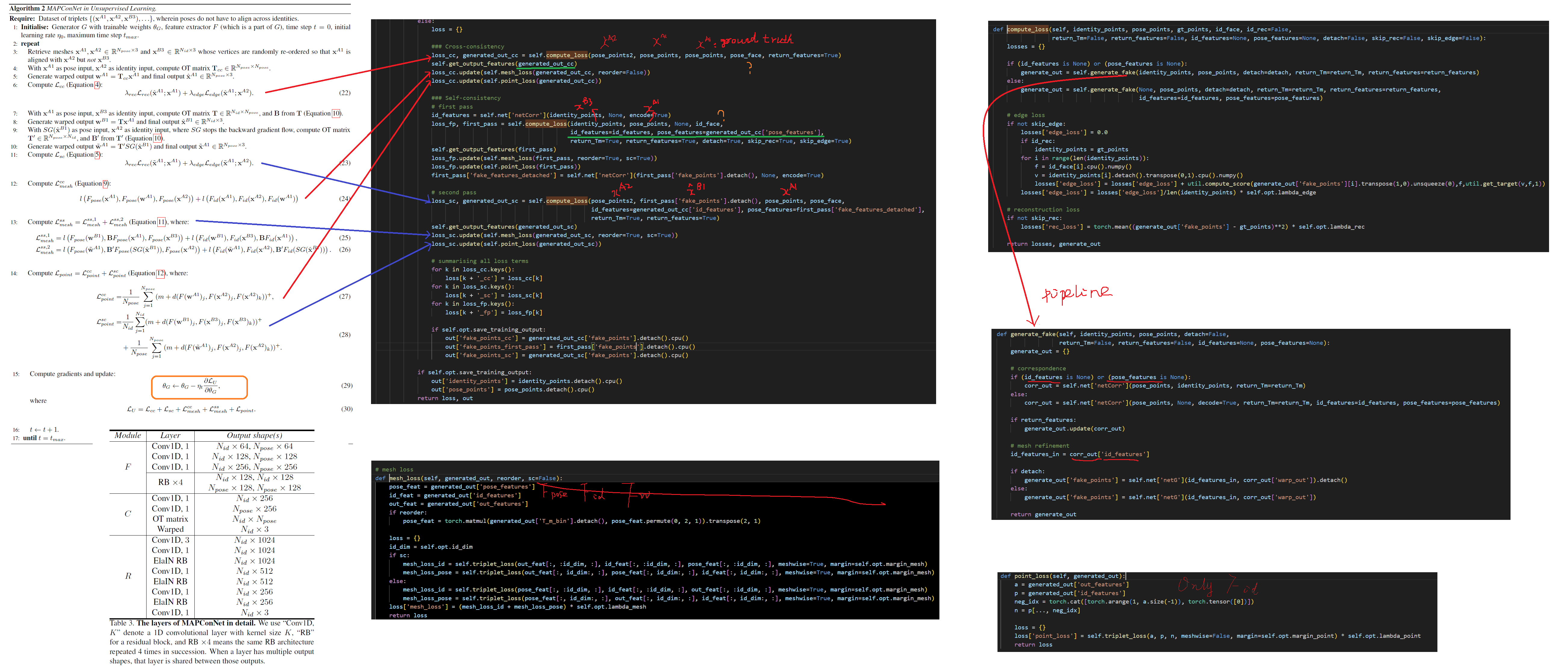
Algorithm
Reference
[47] Keyang Zhou, Bharat Lal Bhatnagar, and Gerard PonsMoll. Unsupervised shape and pose disentanglement for 3D meshes. In The European Conference on Computer Vision (ECCV), August 2020
[33] Chaoyue Song, Jiacheng Wei, Ruibo Li, Fayao Liu, and Guosheng Lin. 3D pose transfer with correspondence learning and mesh refinement. In A. Beygelzimer, Y. Dauphin, P. Liang, and J. Wortman Vaughan, editors, Advances in Neural Information Processing Systems, 2021.
[20] Matthew Loper, Naureen Mahmood, Javier Romero, Gerard Pons-Moll, and Michael J. Black. SMPL: A skinned multi-person linear model. ACM Transaction on Graphics, 34(6):248:1–248:16, Oct. 2015.
[40] Jiashun Wang, Chao Wen, Yanwei Fu, Haitao Lin, Tianyun Zou, Xiangyang Xue, and Yinda Zhang. Neural pose transfer by spatially adaptive instance normalization. In Proceedings of the IEEE/CVF Conference on Computer Vision and Pattern Recognition (CVPR), June 2020.

