Keywords: Discriminant Functions, Logistic Regression, Bayesian Logistic Regression, Python
This is the Chapter4 ReadingNotes from book Bishop-Pattern-Recognition-and-Machine-Learning-2006. [Code_Python]
Discriminant Functions(判别函数)
A discriminant is a function that takes an input vector $\pmb{x}$ and assigns it to one of $K$ classes, denoted $\mathcal{C}_k$.
Linear discriminants, namely those for which the decision surfaces are hyperplanes.
Two classes
The simplest representation of a linear discriminant function is obtained by taking a linear function of the input vector so that
$$
y(\pmb{x}) = \pmb{w^Tx} + w_0
\tag{4.4}
$$
where $\pmb{w}$ is called a weight vector, and $w_0$ is a bias (not to be confused with bias in the statistical sense). The negative of the bias is sometimes called a threshold.
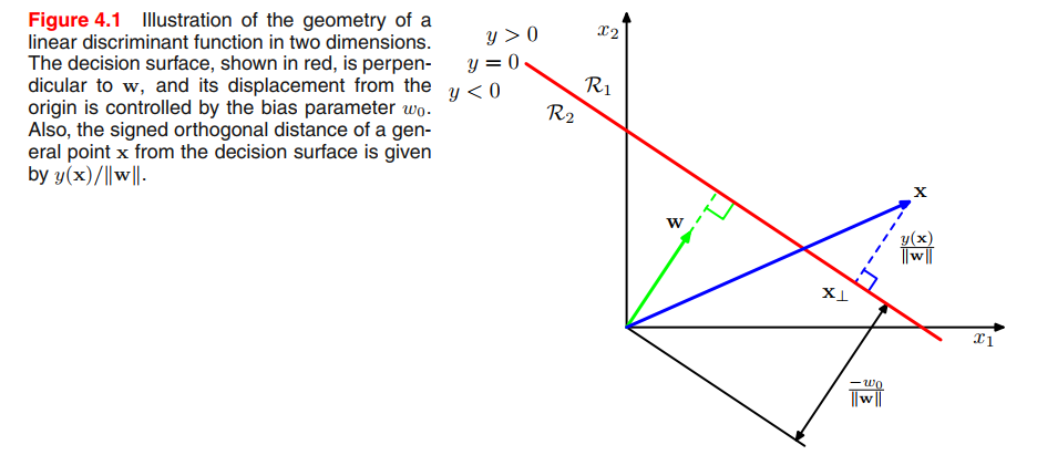
if $\pmb{x}$ is a point on the decision surface, then $y(\pmb{x}) = 0$, and so the normal distance from the origin to the decision surface is given by
$$
\frac{\pmb{w^T}\pmb{x}}{||\pmb{w}||} = -\frac{w_0}{||\pmb{w}||}
\tag{4.5}
$$
$\pmb{w}$ determines the orientation of the decision surface, bias parameter $w_0$ determines the location of the decision surface.
You can understand from 👉surface denotation view $z = f(x,y)$ in Calculus >>
the decision surfaces are $D$-dimensional hyperplanes passing through the origin of the $D + 1$-dimensional expanded input space.
Multiple classes

From Figure 4.2, we can see the ambiguous regions, to avoid this difficulty, we consider a single $K$-class discriminant comprising $K$ linear functions of the form
$$
y_k(\pmb{x}) = \pmb{w_k^Tx} + w_{k0}
\tag{4.9}
$$
and then assigning a point $\pmb{x}$ to class $\mathcal{C}_k$ if $y_k(\pmb{x}) > y_j(\pmb{x})$ for all $j \neq k$.
The decision boundary between class $\mathcal{C}_k$ and class $\mathcal{C}_j$ is therefore given by $y_k(\pmb{x}) = y_j(\pmb{x})$ and hence corresponds to a $(D − 1)$-dimensional hyperplane defined by
$$
(\pmb{w_k - w_j})^T\pmb{x} + (w_{k0} - w_{j0}) = 0
\tag{4.10}
$$
Still imagine the surface $z = f(x,y)$, there are many surfaces in the $R^3$ space, when the two surfaces intersect with each other, means $z_k = z_j$.
The decision regions of such a discriminant are always singly connected and convex.
To see this, consider two points $x_A$ and $x_B$ both of which lie inside decision region $\mathcal{R}_k$, as illustrated in Figure 4.3. Any point $\hat{x}$ that lies on the line connecting $x_A$ and $x_B$ can be expressed in the form
$$
\hat{x} = \lambda x_A + (1-\lambda)x_B, 0 \leq \lambda \leq 1
\tag{4.11}
$$
From the linearity of the discriminant functions, it follows that
$$
y_k(\hat{x}) = \lambda y_k(x_A) + (1-\lambda)y_k(x_B)
\tag{4.12}
$$
Because both $x_A$ and $x_B$ lie inside $\mathcal{R}_k$, it follows that $y_k(x_A) > y_j(x_A)$, and $y_k(x_B) > y_j(x_B)$, for all $j \neq k$, and hence $y_k(\hat{x}) > y_j(\hat{x})$, and so $\hat{x}$ also lies inside $\mathcal{R}_k$. Thus $\mathcal{R}_k$ is singly connected and convex.
👉More About Convex in Algebra>>
Least squares for classification
👉More about Least Squares for Linear Regression >>
Each class $\mathcal{C_k}$ is described by its own linear model so that
$$
y_k(\pmb{x}) = \pmb{w^T_k x} + w_{k0}
\tag{4.13}
$$
where $k = 1, \cdots , K$. We can conveniently group these together using vector notation so that
$$
\pmb{y(x)} = \pmb{\widetilde{W}^T\widetilde{x}}
\tag{4.14}
$$
we obtain the solution for $\widetilde{W}$ in the form
$$
\widetilde{W} = (\widetilde{X}^T\widetilde{X})^{-1}\widetilde{X}^TT
\tag{4.16}
$$
The least-squares approach gives an exact closed-form solution for the discriminant function parameters.
We have already seen that least-squares solutions lack robustness to outliers(对异常值缺乏鲁棒性), and this applies equally to the classification application, as illustrated in Figure 4.4. However, problems with least squares can be more severe than simply lack of robustness, as illustrated in Figure 4.5.
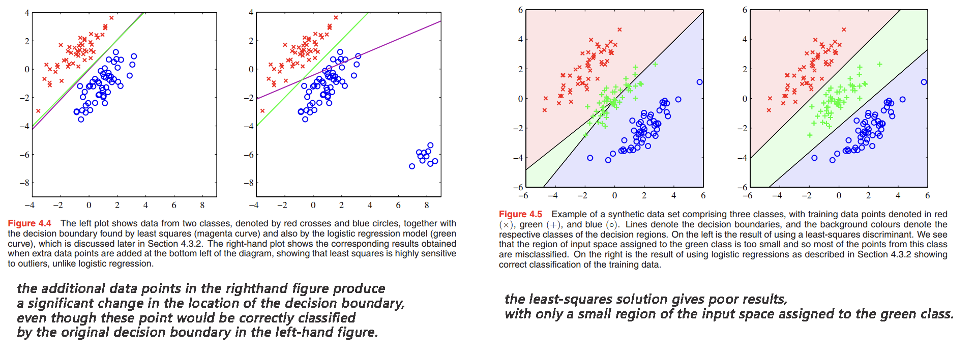
The failure of least squares should not surprise us when we recall that it corresponds to maximum likelihood under the assumption of a Gaussian conditional distribution, whereas binary target vectors clearly have a distribution that is far from Gaussian.
Fisher’s linear discriminant
suppose we take the $D$-dimensional input vector $\pmb{x}$ and project it down to $1$-dimension using
$$
y = \pmb{w^Tx}
\tag{4.20}
$$
In general, the projection onto one dimension leads to a considerable loss of information, and classes that are well separated in the original $D$-dimensional space may become strongly overlapping in $1$- dimension.
consider a two-class problem in which there are $N_1$ points of class $\mathcal{C_1}$ and $N_2$ points of class $\mathcal{C_2}$, so that the mean vectors of the two classes are given by
$$
\pmb{m_1} = \frac{1}{N_1}\sum_{n\in \mathcal{C_1}} \pmb{x_n}\\
\pmb{m_2} = \frac{1}{N_2}\sum_{n\in \mathcal{C_2}} \pmb{x_n}
\tag{4.21}
$$
The simplest measure of the separation of the classes, when projected onto $\pmb{w}$, is the separation of the projected class means. This suggests that we might choose $\pmb{w}$ so as to maximize
$$
m_2 - m_1 = \pmb{w^T}(\pmb{m_2 - m_1})
\tag{4.22}
$$
where,
$$
m_k = \pmb{w^Tm_k}
\tag{4.23}
$$
is the mean of the projected data from class $\mathcal{C_k}$.
Using a 👉Lagrange multiplier >> to perform the constrained maximization, the constrained condition is $\sum_{i} w_i^2 = 1$, we then find that
$$
\pmb{w} \propto \pmb{(m_2 − m_1)}
$$

The within-class variance of the transformed data from class $\mathcal{C_k}$ is therefore given by
$$
s_k^2 = \sum_{n \in \mathcal{C_k}} (y_n - m_k)^2, y_n = \pmb{w^Tx_n}
\tag{4.24}
$$
total within-class variance for the whole data set is
$$
s_1^2 + s_2^2
$$
The Fisher criterion is defined to be the ratio of the between-class variance to the within-class variance and is given by
$$
J(\pmb{w}) = \frac{(m_2 - m_1)^2}{s_1^2 + s_2^2}
\tag{4.25}
$$
By equation (4.20), (4.23), (4.24), we get
$$
J(\pmb{w}) = \frac{\pmb{w^TS_Bw}}{\pmb{w^TS_Ww}}
\tag{4.26}
$$
where $\pmb{S_B}$ is the between-class covariance matrix and is given by
$$
\pmb{S_B} = (\pmb{m_2 - m_1})(\pmb{m_2 - m_1})^T
\tag{4.27}
$$
$\pmb{S_W}$ is the total within-class covariance matrix, given by
$$
\pmb{S_W} = \sum_{n \in \mathcal{C_1}}\pmb{(x_n - m_1)(x_n - m_1)^T} + \sum_{n \in \mathcal{C_2}}\pmb{(x_n - m_2)(x_n - m_2)^T}
\tag{4.28}
$$
Differentiating (4.26) with respect to $\pmb{w}$, we find that $J(\pmb{w})$ is maximized when
$$
\pmb{(w^TS_Bw)S_Ww} = \pmb{(w^TS_Ww)S_Bw}
\tag{4.29}
$$
we get
$$
\pmb{w} \propto \pmb{S_W^{-1}(m_2-m_1)}
\tag{4.30}
$$
if the within-class covariance is isotropic, so that $\pmb{S_W}$ is proportional to the unit matrix, we find that $\pmb{w}$ is proportional to the difference of the class means, as discussed above.
Relation to least squares
Fisher’s discriminant for multiple classes
$$
J(\pmb{w}) = Tr \lbrace (\pmb{WS_WW^T})^{-1} (\pmb{WS_BW^T})\rbrace
\tag{4.51}
$$
The perceptron algorithm
The general of perceptron algorithm is
$$
y(\pmb{x}) = f(\pmb{w^T}\phi(\pmb{x}))
\tag{4.52}
$$
where the nonlinear activation function $f(\cdot)$ is given by a step function of the form
$$
f(a) =
\begin{cases}
+1, a \geq 0\\
-1, a < 0
\end{cases}
\tag{4.53}
$$
it is more convenient to use target values $t = +1$ for class $\mathcal{C_1}$ and $t = −1$ for class $\mathcal{C_2}$, which matches the choice of activation function.
We consider an alternative error function known as the perceptron criterion:
$$
E_P(\pmb{w}) = - \sum_{n \in \mathcal{M}} \pmb{w^T}\phi_n t_n
\tag{4.54}
$$
where $\mathcal{M}$ denotes the set of all misclassified patterns.
We now apply the stochastic gradient descent algorithm to this error function. The change in the weight vector $\pmb{w}$ is then given by
$$
\pmb{w}^{(\tau + 1)} = \pmb{w}^{(\tau)} - \eta \nabla E_p(\pmb{w}) = \pmb{w}^{(\tau)} + \eta \phi_n t_n
\tag{4.55}
$$
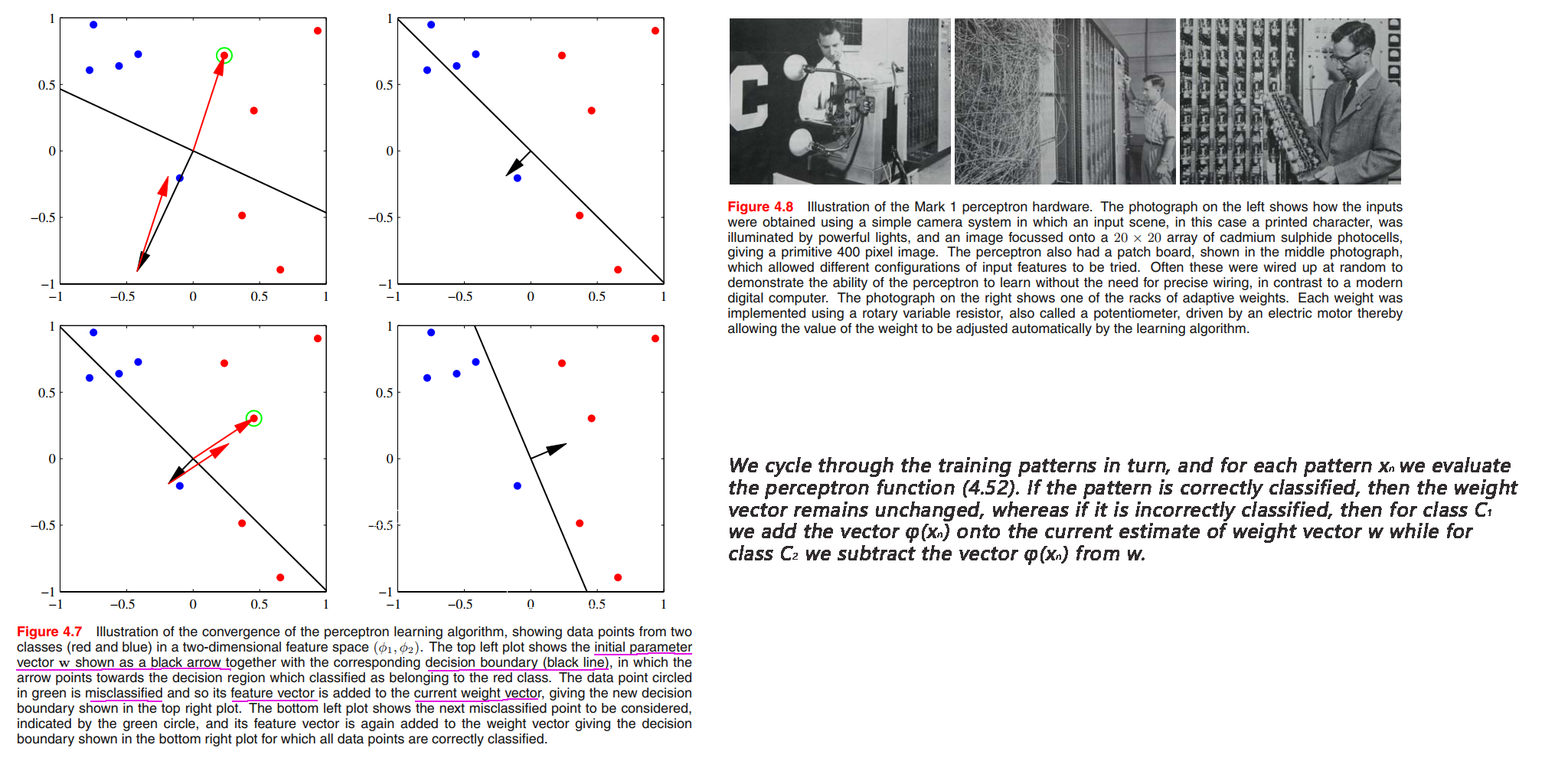
Furthermore, for data sets that are not linearly separable, the perceptron learning algorithm will never converge.
Probabilistic Generative Models
Here we shall adopt a generative approach in which we model the class-conditional densities $p(\pmb{x} | C_k)$, as well as the class priors $p(C_k)$, and then use these to compute posterior probabilities $p(C_k|\pmb{x})$ through Bayes’ theorem.
Consider first of all the case of two classes. The posterior probability for class $C_1$ can be written as
$$
p(C_1 | \pmb{x}) = \frac{p(\pmb{x} | C_1) p(C_1)}{p(\pmb{x} | C_1) p(C_1) + p(\pmb{x} | C_2) p(C_2)} = \frac{1}{1 + exp(-a)} = \sigma(a)
\tag{4.57}
$$
where
$$
a = \ln \frac{p(\pmb{x} | C_1) p(C_1)}{p(\pmb{x} | C_2) p(C_2)}
\tag{4.58}
$$
For the case of $K > 2$ classes, we have
$$
p(C_k | \pmb{x}) = \frac{p(\pmb{x} | C_k) p(C_k)}{\sum_j p(\pmb{x} | C_j) p(C_j)} = \frac{exp(a_k)}{\sum_j exp(a_j)}
\tag{4.62}
$$
The normalized exponential is also known as the softmax function, as it represents a smoothed version of the ‘max’ function because, if $a_k >> a_j$ for all $j \neq k$, then $p(C_k|\pmb{x}) \simeq 1$, and $p(C_j|\pmb{x}) \simeq 0$.
Continuous inputs
Assume the class-conditional densities are Gaussian and then explore the resulting form for the posterior probabilities. The density for class $C_k$ is given by
$$
p(\pmb{x} | C_k) = \frac{1}{(2\pi)^{D/2}}\frac{1}{|\Sigma|^{1/2}} exp \lbrace -\frac{1}{2} (\pmb{x - \mu_k})^T \Sigma^{-1} \pmb{x - \mu_k}\rbrace
\tag{4.64}
$$
From (4.57) and (4.58), we have
$$
p(C_1 | \pmb{x}) = \sigma(\pmb{w^T x} + w_0)
\tag{4.65}
$$
where we have defined
$$
\pmb{w} = \Sigma^{-1} (\pmb{\mu_1 - \mu_2})
\tag{4.66}
$$
$$
w_0 = -\frac{1}{2} \pmb{\mu_1}^T \Sigma^{-1} \pmb{\mu_1} + \frac{1}{2} \pmb{\mu_2}^T \Sigma^{-1} \pmb{\mu_2} + \ln \frac{p(C_1)}{p(C_2)}
\tag{4.67}
$$
For the general case of K classes we have, from (4.62) and (4.63),
$$
a_k(\pmb{x}) = \pmb{w_k}^T\pmb{x} + w_{k0}
\tag{4.68}
$$
where we have defined
$$
\pmb{w} = \Sigma^{-1} (\pmb{\mu_k})
\tag{4.69}
$$
$$
w_0 = -\frac{1}{2} \pmb{\mu_k}^T \Sigma^{-1} \pmb{\mu_k} + \ln p(C_k)
\tag{4.70}
$$

Maximum likelihood solution
Once we have specified a parametric functional form for the class-conditional densities $p(\pmb{x}|C_k)$, we can then determine the values of the parameters, together with the prior class probabilities $p(C_k)$, using maximum likelihood. This requires a data set comprising observations of $x$ along with their corresponding class labels.
就是说现在还是最大似然函数那一套:先建模,比如用高斯去参数化model,然后点估计,最大化似然函数得到参数 $w_{ML}$
Consider first the case of two classes, each having a Gaussian class-conditional density with a shared covariance matrix, and suppose we have a data set $\lbrace x_n, t_n \rbrace$ where $n = 1, \cdots , N$. Here $t_n = 1$ denotes class $C_1$ and $t_n = 0$ denotes class $C_2$. We denote the prior class probability $p(C_1) = \pi$, so that $p(C_2) = 1−\pi$. For a data point $x_n$ from class $C_1$, we have $t_n = 1$ and hence
$$
p(x_n, C_1) = p(C_1)p(x_n | C_1) = \pi N(x_n | \mu_1, \Sigma)
$$
Thus the likelihood function is given by
$$
p(T|\pi, \mu_1, \mu_2, \Sigma) = \prod_{n=1}^{N} [\pi N(x_n | \mu_1, \Sigma)]^{t_n}[(1-\pi)N(x_n | \mu_2, \Sigma)]^{1-t_n}
\tag{4.71}
$$
maximum the log of likelihood function we get,
$$
\pi = \frac{N_1}{N_1 + N_2}
\tag{4.73}
$$
where $N_1$ denotes the total number of data points in class $C_1$, and $N_2$ denotes the total number of data points in class $C_2$.
$$
\mu_1 = \frac{1}{N_1} \sum_{n=1}^N t_n x_n
\tag{4.75}
$$
which is simply the mean of all the input vectors $x_n$ assigned to class $C_1$. Similar,
$$
\mu_2 = \frac{1}{N_2} \sum_{n=1}^N (1 - t_n) x_n
\tag{4.76}
$$
Also, we have
$$
\Sigma = S = \frac{N_1}{N} S_1 + \frac{N_2}{N} S_2
\tag{4.78}
$$
where
$$
S_1 = \frac{1}{N_1} \sum_{n \in C_1} (x_n - \mu_1) (x_n - \mu_1)^T
\tag{4.79}
$$
$$
S_1 = \frac{1}{N_2} \sum_{n \in C_2} (x_n - \mu_2) (x_n - \mu_2)^T
\tag{4.80}
$$
Discrete features
Exponential family
Probabilistic Discriminative Models
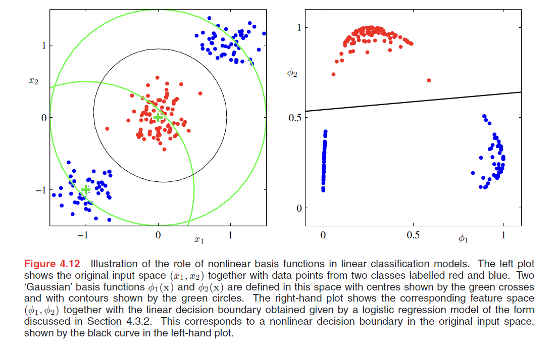
Fixed basis functions
Logistic regression
In our discussion of generative approaches before, we saw that under rather general assumptions, the posterior probability of class $C_1$ can be written as a logistic sigmoid acting on a linear function of the feature vector $\phi$ so that
$$
p(C_1 | \phi) = y(\phi) = \sigma(\pmb{w^T} \phi)
\tag{4.87}
$$
Here $\sigma(·)$ is the logistic sigmoid function defined by (4.59). In the terminology of statistics, this model is known as logistic regression, although it should be emphasized that this is a model for classification rather than regression.
$$
\sigma(a) = \frac{1}{1 + exp(-a)}
\tag{4.59}
$$
We now use maximum likelihood to determine the parameters of the logistic regression model.
For a dataset $\lbrace \phi_n, t_n\rbrace$, where $t_n \in \lbrace 0,1\rbrace$, and $\phi_n = \phi(x_n)$, with $n = 1, \cdots, N$. The likelyhood function is
$$
p(T|\pmb{w}) = \prod_{n=1}^{N} y_n^{t_n} \lbrace 1 - y_n\rbrace^{1-t_n}
\tag{4.89}
$$
where
$$
y_n = p(C_1|\phi_n)
$$
As usual, crossentropy error function in the form
$$
\begin{aligned}
E(\pmb{w}) &= -\ln p(T|\pmb{w}) \\
&= -\sum_{n=1}^{N} \lbrace t_n \ln y_n + (1-t_n)\ln(1-y_n)\rbrace
\end{aligned}
\tag{4.90}
$$
where
$$
y_n = \sigma(a_n)
$$
and
$$
a_n = \pmb{w}^T\phi_n
$$
Taking the gradient of the error function with respect to $\pmb{w}$, we obtain
$$
\nabla E(\pmb{w}) = \sum_{n=1}^N (y_n - t_n)\phi_n
\tag{4.91}
$$
comparison with (3.13) shows that this takes precisely the same form as the gradient of the sum-of-squares error function for the linear regression model.
$$
\nabla \ln p(T|\pmb{w},\beta) = \sum_{n=1}^N \lbrace t_n - \pmb{w^T}\phi(x_n)\rbrace \phi(x_n)^T
\tag{3.13}
$$
Iterative reweighted least squares
In the case of the linear regression models discussed in Chapter 3, the maximum likelihood solution, on the assumption of a Gaussian noise model, leads to a closed-form solution. This was a consequence of the quadratic dependence of the log likelihood function on the parameter vector $w$.
For logistic regression, there is no longer a closed-form solution, due to the nonlinearity of the logistic sigmoid function.
However, the departure from a quadratic form is not substantial. To be precise, the error function is concave, as we shall see shortly, and hence has a unique minimum.
Furthermore, the error function can be minimized by an efficient iterative technique based on the Newton-Raphson iterative optimization scheme, which uses a local quadratic approximation to the log likelihood function.
$$
\pmb{w}^{(new)} = \pmb{w}^{(old)} - \pmb{H}^{-1} \nabla E(\pmb{w})
\tag{4.92}
$$
Here we compare logistic regression with linear regression.
- For Linear Regression
$$
E_D(\pmb{w}) = \frac{1}{2} \sum_{n=1}^{N}\lbrace t_n - \pmb{w^T}\phi(x_n)\rbrace^2
\tag{3.12}
$$
The gradient and Hessian of this error function are given by
$$
\nabla E(\pmb{w}) = \sum_{n=1}^{N}(\pmb{w}^T \phi_n - t_n) \phi_n = \pmb{\Phi^T\Phi w - \Phi^T T}
\tag{4.93}
$$
$$
\pmb{H} = \nabla \nabla E(\pmb{w}) = \sum_{n=1}^{N} \phi_n \phi_n^T = \pmb{\Phi^T\Phi}
\tag{4.94}
$$
The Newton-Raphson update then takes the form
$$
\pmb{w}^{(new)} = \pmb{(\Phi^T \Phi)^{-1} \Phi T}
$$
which we recognize as the standard least-squares solution.
- For Logistic Regression
$$
\nabla E(\pmb{w}) = \sum_{n=1}^N (y_n - t_n)\phi_n = \pmb{\Phi^T(y-t)}
\tag{4.96}
$$
$$
\pmb{H} = \nabla \nabla E(\pmb{w}) = \sum_{n=1}^N y_n(1-y_n)\phi_n \phi_n^T = \pmb{\Phi^TR\Phi}
\tag{4.97}
$$
where
$$
R_{nn} = y_n(1-y_n)
\tag{4.98}
$$
The Newton-Raphson update then takes the form
$$
\pmb{w}^{(new)} = \pmb{(\Phi^T R \Phi)^{-1} \Phi^T R z}
\tag{4.99}
$$
where
$$
\pmb{z} = \pmb{\Phi w}^{(old)} - \pmb{R^{-1}(y-T)}
$$
Because the weighing matrix $\pmb{R}$ is not constant but depends on the parameter vector $\pmb{w}$, we must apply the normal equations iteratively, each time using the new weight vector $\pmb{w}$ to compute a revised weighing matrix $\pmb{R}$. For this reason, the algorithm is known as iterative reweighted least squares, or IRLS (Rubin, 1983).
Multiclass logistic regression
also called softmax regression. The same with two-class logistic regression.
maximum likelihood function–> get the error function–> use Newton-Raphson iterative method –> get unique minimum.
Probit regression
Canonical link functions
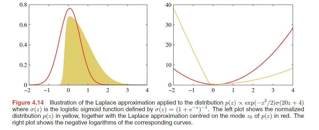
The Laplace Approximation
Recall Bayesian Linear Regression in Chapter3, the posterior distribution is still a Gaussian distribution, but it’s not the same with Bayesian Logistic Regression.
In particular, we cannot integrate exactly over the parameter vector $\pmb{w}$ since the posterior distribution is no longer Gaussian. It is therefore necessary to introduce some form of approximation.
Consider first the case of a single continuous variable $z$, and suppose the distribution $p(z)$ is defined by
$$
p(z) = \frac{1}{Z}f(z)
\tag{4.125}
$$
where $Z = \int f(z) dz$ is the normalization coefficient.
In the Laplace method the goal is to find a Gaussian approximation $q(z)$ which is centred on a mode of the distribution $p(z)$.
The first step is to find a mode of $p(z)$, in other words a point $z_0$ such that $p’(z_0) = 0$, or equivalently
$$
\frac{d f(z)}{dz} |_{z = z_0} = 0
\tag{4.126}
$$
Now we know $z_0$ is a local maximum of the distribution, so if we make a Taylor expansion of $\ln f(z)$ centered on the mode $z_0$, we get
$$
\ln f(z) \simeq \ln f(z_0) - \frac{1}{2}A(z - z_0)^2
$$
for M-dimensional space $\pmb{z}$, we have
$$
\ln f(\pmb{z}) \simeq \ln f(\pmb{z_0}) - \frac{1}{2} \pmb{(z - z_0)}^T \pmb{A} (\pmb{z - z_0})
\tag{4.131}
$$
where
$$
A = -\frac{d^2}{dz^2} \ln f(z) | _{z = z_0}
$$
the $M \times M$ Hessian Matrix $\pmb{A}$ is
$$
\pmb{A} = - \nabla \nabla \ln f(\pmb{z}) | _{\pmb{z = z_0}}
\tag{4.132}
$$
the first-order term does not appear because the first-order at $z_0$ is zero.
Taking the exponential we obtain
$$
f(z) \simeq f(z_0) exp \lbrace -\frac{A}{2}(z-z_0)^2 \rbrace
$$
for vector space we get
$$
f(\pmb{z}) \simeq f(\pmb{z_0}) exp \lbrace -\frac{1}{2} \pmb{(z - z_0)}^T \pmb{A} (\pmb{z - z_0})\rbrace
\tag{4.133}
$$
We can then obtain a normalized distribution $q(z)$ by making use of the standard result for the normalization of a Gaussian, so that
$$
q(z) = (\frac{A}{2\pi})^{1/2} exp \lbrace -\frac{A}{2}(z-z_0)^2\rbrace
$$
using the standard result (2.43) for a normalized multivariate Gaussian, giving
$$
\mathcal{N}(\pmb{x} | \pmb{\mu}, \pmb{\Sigma}) = \frac{1}{(2\pi)^{D/2}}\frac{1}{|\pmb{\Sigma}|^{1/2}} exp \lbrace -\frac{1}{2}(\pmb{x - \mu})^T \pmb{\Sigma}^{-1}(\pmb{x-\mu}) \rbrace
\tag{2.43}
$$
$$
q(\pmb{z}) = \frac{|\pmb{A}^{1/2}|}{(2\pi)^{M/2}} exp \lbrace -\frac{1}{2} (\pmb{z - z_0})^T \pmb{A} (\pmb{z - z_0})\rbrace = N(\pmb{z} | \pmb{z_0, A^{-1}})
\tag{4.134}
$$
This Gaussian distribution will be well defined provided its precision matrix, given by $\pmb{A}$, is positive definite, which implies
that the stationary point $\pmb{z_0}$ must be a local maximum, not a minimum or a saddle point. (👉Recall Extrema in Calculus >>)
Model comparison and BIC
As well as approximating the distribution $p(\pmb{z})$ we can also obtain an approximation to the normalization constant $Z$. Using the approximation (4.133) we have
$$
\begin{aligned}
Z &= \int f(\pmb{z}) d\pmb{z} \\
& \simeq f(\pmb{z_0}) \int exp \lbrace -\frac{1}{2} \pmb{(z - z_0)}^T \pmb{A} (\pmb{z - z_0})\rbrace d\pmb{z} \\
&= f(\pmb{z_0}) \frac{(2\pi)^{M/2}}{|\pmb{A}|^{1/2}}
\end{aligned}
\tag{4.135}
$$
Bayesian Logistic Regression
Laplace approximation
Because we seek a Gaussian representation for the posterior distribution, it is natural to begin with a Gaussian prior, which we write in the general form
$$
p(\pmb{w}) = N(\pmb{w} | \pmb{m_0, S_0})
\tag{4.140}
$$
The posterior distribution over $\pmb{w}$ is given by
$$
p(\pmb{w | t}) \propto p(\pmb{w}) p(\pmb{t | w})
\tag{4.141}
$$
where $\pmb{t} = (t_1, \cdots , \pmb{t_N})^T$.
(4.140) and (4.89), take the log of both sides, we get
$$
\ln p(\pmb{w|t}) = -\frac{1}{2}(\pmb{w - m_0})^T \pmb{S_0}^{-1} (\pmb{w - m_0}) + \sum_{n=1}^{N} \lbrace t_n \ln y_n + (1 - t_n) \ln (1-y_n)\rbrace + const
\tag{4.142}
$$
where $y_n = \sigma(\pmb{w}^T \phi_n)$
To obtain a Gaussian approximation to the posterior distribution, we first maximize the posterior distribution to give the MAP (maximum posterior) solution $\pmb{w_{MAP}}$, which defines the mean of the Gaussian.
The covariance is then given by the inverse of the matrix of second derivatives of the negative log likelihood, which takes the form
$$
\pmb{S_N} = - \nabla \nabla \ln p(\pmb{w|t}) = \pmb{S_0}^{-1} + \sum_{n=1}^{N} y_n(1-y_n)\phi_n \phi_n^T
\tag{4.143}
$$
The Gaussian approximation to the posterior distribution therefore takes the form
$$
q(\pmb{w}) = N(\pmb{w} | \pmb{w_{MAP}, S_N})
\tag{4.144}
$$
Predictive distribution
The predictive distribution for class $C_1$, is
$$
p(C_1 | \phi, \pmb{t}) = \int p(C_1 | \phi, \pmb{w}) p(\pmb{w|t}) d\pmb{w} \simeq \int \sigma(\pmb{w}^T \phi) q(\pmb{w}) d\pmb{w}
\tag{4.145}
$$
…
we get
$$
p(C_1 | \phi, \pmb{t}) = \sigma(\kappa(\sigma_a^2)\mu_a)
\tag{4.155}
$$
where
$$
\kappa (\sigma^2) = (1 + \pi \sigma^2 / 8)^{-1/2}
\tag{4.154}
$$
$$
\mu_a = \pmb{w}_{MAP}^T \phi
\tag{4.149}
$$
$$
\sigma_a^2 = \phi^T \pmb{S_N} \phi
\tag{4.150}
$$

