Keywords: Aumented matrix, Linear Independence, Linear Transformation
This is the Chapter1 ReadingNotes from book Linear Algebra and its Application.
System of Linear Equations
Linear Equation:
$$
a_1 x_1 + a_2 x_2 + … + a_n x_n = b
$$
NonLinear Equation:
$$
4 x_1 - 5 x_2 = x_1x_2
$$
Linear System
$$
\begin{cases}
&2 x_1 - x_2 + 1.5 x_3 = 8 \\
&x_1 - 4 x_3 = -7
\end{cases}
\tag{2}
$$
Solution set
The set of all possible solutions is called the solution set of the linear system.
e.g. (5, 6.5, 3) is a solution of system(2)
Two linear systems are called equivalent if they have the same solution set.
A system of linear equations has
- no solution, or
- exactly one solution, or
- infinitely many solutions
Augmented Matrix
$$
\begin{cases}
x_1 - 2 x_2 + x_3 = 0\\
2x_2 - 8x_3 = 8 \\
5x_1 - 5x_3 = 10
\end{cases}
\rightarrow
\begin{bmatrix}
1 & -2 & 1 & 0 \\
0 & 2 & -8 & 8\\
5 & 0 & -5 & 10
\end{bmatrix}
$$
Solving a Linear System
The procedure can also be called simplify the augmented matrix
(化简增广矩阵的过程就是在求线性方程组的解)
$$
\begin{cases}
x_1 = 1, \\x_2 = 0, \\x_3 = -1
\end{cases}
\rightarrow
\begin{bmatrix}
1 & 0 & 0 & 1 \\
0 & 1 & 0 & 0\\
0 & 0 & 1 & -1
\end{bmatrix}
$$
ELEMENTARY ROW OPERATIONS
- (Replacement) Replace one row by the sum of itself and a multiple of another row
- (Interchange) Interchange two rows.
- (Scaling) Multiply all entries in a row by a nonzero constant
Existence and Uniqueness Questions
this system solution is unique, this system is consistent:
$$
\begin{cases}
x_1 - 2 x_ 2 + x_3 = 0\\
x_2 - 4x_3 = 4\\
x_3 = -1
\end{cases}
\rightarrow
\begin{bmatrix}
1 & -2 & 1 & 0 \\
0 & 1 & -4 & 4\\
0 & 0 & 1 & -1
\end{bmatrix}
$$
Row Reduction and Echelon Forms
a nonzero row or column
a row or column that contains at least one nonzero entry
leading entry
a leading entry of a row refers to the leftmost nonzero entry (in a nonzero row)
A rectangular matrix is in echelon form (or row echelon form) if it has the following three properties:
- All nonzero rows are above any rows of all zeros.
- Each leading entry of a row is in a column to the right of the leading entry of the row above it.
- All entries in a column below a leading entry are zeros.
If a matrix in echelon form satisfies the following additional conditions, then it is in reduced echelon form (or reduced row echelon form):- The leading entry in each nonzero row is 1.
- Each leading 1 is the only nonzero entry in its column.
行阶梯矩阵 row echelon form
$$
\begin{bmatrix}
2 & -3 & 2 & 1 \\
0 & 1 & -4 & 8\\
0 & 0 & 0 & 5/2
\end{bmatrix}
$$
最简阶梯矩阵 reduced echelon form
$$
\begin{bmatrix}
1 & 0 & 0 & 29 \\
0 & 1 & 0 & 16\\
0 & 0 & 1 & 3
\end{bmatrix}
$$
Pivot Positons
A pivot position in a matrix A is a location in A that corresponds to a leading 1
in the reduced echelon form of A. A pivot column is a column of A that contains
a pivot position
I think the leading entry is pivot postion.
只是pivot postions是在最简阶梯矩阵的语境下的
Solutions of Linear Systems
The variables $x_1$ and $x_2$ corresponding to pivot columns in the matrix are called basic variables.
The other variable, $x_3$, is called a free variable.
$$
\begin{cases}
x_1 - 5 x_ 3 = 1 \\
x_2 + x_3 = 4\\
0 = 0
\end{cases}
\rightarrow
\begin{bmatrix}
1 & 0 & -5 & 1 \\
0 & 1 & 1 & 4\\
0 & 0 & 0 & 0
\end{bmatrix}
$$
Augumented matrix has solution
Existence and Uniqueness Theorem
A linear system is consistent if and only if the rightmost column of the augmented matrix is not a pivot column—that is, if and only if an echelon form of the augmented matrix has no row of the form
$$
\begin{bmatrix}0 & \cdots &0 & b\end{bmatrix} with \space b\space nonzero
$$
If a linear system is consistent, then the solution set contains either (i) a unique solution, when there are no free variables, or (ii) infinitely many solutions, when there is at least one free variable.
Vector Equations
Vector in $R^n$
if $n$ is a positive integer, $R^n$ denotes the collection of all lists (or ordered n-tuples) of $n$ real numbers, usually written as $n \times 1$ column matrics, such as
$$
\vec{a} = \begin{bmatrix} u_1\\u_2\\\cdots\\u_3\end{bmatrix}
$$
Linear Combinations
Given vectors $\vec{v_1}, \vec{v_2}, \cdots, \vec{v_p}$ in $R^n$ and given scalars $c_1, c_2, \cdots, c_p$, the vector $\vec{y}$ defined by
$$
\vec{y} = c_1\vec{v_1} + \cdots + c_p\vec{v_p}
$$
is called a linear combination of $\vec{v_1}, \cdots, \vec{v_p}$ with weights $c_1, \cdots, c_p$
Linear Combinations & Matrics
A vector equation
$$
x_1\vec{a_1} + x_2\vec{a_2} + \cdots + x_n\vec{a_n} = \vec{b}
$$
has the same solution set as the linear system whose augmented matrix is
$$
\begin{bmatrix}\vec{a_1} & \vec{a_2} & \cdots & \vec{a_n} & \vec{b}\end{bmatrix}
\tag{5}
$$
In particular, $\vec{b}$ can be generated by a linear combination of $\vec{a_1}\cdots\vec{a_n}$ if and only if there exists a solution to the linear system corresponding to the matrix(5)
Span{$\vec{v_1}, \cdots, \vec{v_p}$}
Asking whether a vector $\vec{b}$ is in Span{$\vec{v_1}, \cdots, \vec{v_p}$} amounts to asking whether the vector equation
$$
x_1\vec{v_1} + \cdots + x_p\vec{v_p} = \vec{b}
$$
has a solution, or, equivalently, asking whether the linear system with augmented matrix
$$
\begin{bmatrix}\vec{v_1} & \cdots & \vec{v_p} & \vec{b}\end{bmatrix}
$$
has a solution
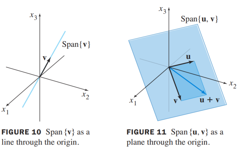
A Geometric Description of Span{$\vec{v}$} and Span{$\vec{u}, \vec{v}$}
Let $\vec{v}$ be a nonzero vector in $R^3$. Then Span{$\vec{v}$} is the set of all scalar multiples of $\vec{v}$, which is the set of points on the line in $R^3$ through $\vec{v}$ and $\vec{0}$. See Figure 10.
If $\vec{u}$ and $\vec{v}$ are nonzero vectors in $R^3$, with $\vec{v}$ not a multiple of $\vec{u}$, then Span{$\vec{u},\vec{v}$}is the plane in $R^3$ that contains $\vec{u}$, $\vec{v}$, and $\vec{0}$. In particular, Span{$\vec{u},\vec{v}$} contains the line in $R^3$ through $\vec{u}$ and $\vec{0}$ and the line through $\vec{v}$ and $\vec{0}$. See Figure 11.
The Matrix Equation $Ax = b$
if $A$ is an $m \times n$ matrix, with columns $\vec{a_1}, \cdots, \vec{a_n}$, and if $\vec{x}$ is in $R^n$, then the product of $A$ and $\vec{x}$, denoted by $A\vec{x}$, is the linear combination of the columns of $A$ using the corresponding entries in $\vec{x}$ as weights; that is,
$$
A\vec{x} =
\begin{bmatrix}\vec{a_1} & \vec{a_2} & \cdots \vec{a_n}\end{bmatrix}
\begin{bmatrix}x_1\\ \cdots \\ x_n\end{bmatrix}
=x_1\vec{a_1}+x_2\vec{a_2}+\cdots+x_n\vec{a_n}
$$
以下四种写法是等价的,全部转化为求增广矩阵的Solution:
$$
\begin{cases}
x_1 + 2x_2 - x_3 = 4\\
-5x_2 + 3x_3 = 1 \tag{1}
\end{cases}
$$
$$
x_1
\begin{bmatrix}
1\\0
\end{bmatrix} +
x_2
\begin{bmatrix}
2\\-5
\end{bmatrix} +
x_3
\begin{bmatrix}
-1\\3
\end{bmatrix} =
\begin{bmatrix}
4\\1
\end{bmatrix} \tag{2}
$$
$$
\begin{bmatrix}
1 & 2 & -1\\
0 & -5 & 3
\end{bmatrix}
\begin{bmatrix}
x_1\\x_2\\x_3
\end{bmatrix}
=
\begin{bmatrix}
4 \\ 1
\end{bmatrix} \tag{3}
$$
$$
\begin{bmatrix}
1 & 2 & -1 & 4\\
0 & -5 & 3 & 1
\end{bmatrix} \tag{4}
$$
计算机存储矩阵,用连续的空间存储提高效率
To optimize a computer algorithm to compute $Ax$, the sequence of calculations
should involve data stored in contiguous memory locations. The most widely
used professional algorithms for matrix computations are written in Fortran, a
language that stores a matrix as a set of columns. Such algorithms compute $Ax$ as
a linear combination of the columns of $A$. In contrast, if a program is written in
the popular language C, which stores matrices by rows, Ax should be computed
via the alternative rule that uses the rows of $A$
Solution sets of linear systems
Homogeneous Linear Systems
A system of linear equations is said to be homogeneous if it can be written in the form $A\vec{x} = 0 $, where A is an $m \times n$ matrix and $\vec{0}$ is the zero vector in $R^m$.
$\vec{x} = \vec{0}$ is a trivial solution.
The homogeneous equation $A\vec{x} = 0 $ has a nontrivial solution if and only if the equation has at least one free variable.
💡For Example💡:
$$
\begin{cases}
3x_1 + 5x_2 - 4x_3 = 0\\
-3x_1 - 2x_2 + 4x_3 = 0\\
6x_1 + x_2 - 8x_3 = 0 \tag{1}
\end{cases}
$$
Solution:
$$
\begin{bmatrix}
3 & 5 & -4 & 0\\
-3 & 2 & 4 & 0\\
6 & 1 & -8 & 0
\end{bmatrix}
\sim
\begin{bmatrix}
3 & 5 & -4 & 0\\
0 & 3 & 0 & 0\\
0 & -9 & 0 & 0
\end{bmatrix}
\sim
\begin{bmatrix}
3 & 5 & -4 & 0\\
0 & 3 & 0 & 0\\
0 & 0 & 0 & 0
\end{bmatrix}
$$
Since $x_3$ is a free variable, $A\vec{x} = \vec{0}$ has nontrivial solutions, continue the row reduction of $\begin{bmatrix}A & \vec{0}\end{bmatrix}$ to reduced echelon form:
$$
\begin{bmatrix}
1 & 0 & -4/3 & 0\\
0 & 3 & 0 & 0\\
0 & 0 & 0 & 0
\end{bmatrix}
\rightarrow
\begin{matrix}x_1-\frac{4}{3}x_3 = 0\\
x_2 = 0\\
0 = 0\end{matrix}
$$
the general solution of $A\vec{x} = \vec{0}$ has the form:
$$
\vec{x} = \begin{bmatrix}
x_1\\x_2\\x_3
\end{bmatrix}
=
\begin{bmatrix}
\frac{4}{3}x_3\\0\\x_3
\end{bmatrix}
=
x_3\begin{bmatrix}
\frac{4}{3}\\0\\1
\end{bmatrix}
=
x_3\vec{v},
where\space \vec{v} = \begin{bmatrix}\frac{4}{3}\\0\\1\end{bmatrix}
$$
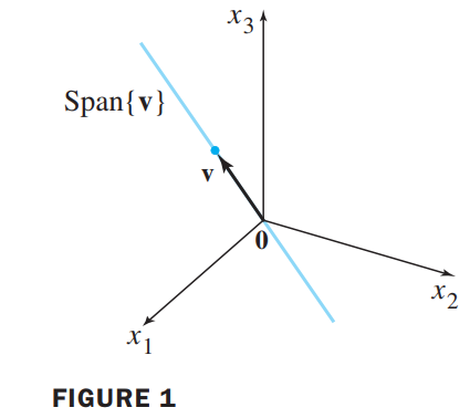
Geometrically, the solution set is a line through $\vec{0}$ in $R^3$. See Figure1.
Also, form as $\vec{x} = x_3\vec{v}$, we say that the solution is in parametric vector form.
Solutions of Nonhomogeneous Linear Systems
💡For example💡:
$$
\begin{bmatrix}
3 & 5 & -4 & 7\\
-3 & -2 & 4 & -1\\
6 & 1 & -8 & -4
\end{bmatrix}
\sim
\begin{bmatrix}
1 & 0 & -4/3 & -1\\
0 & 1 & 0 & 2\\
0 & 0 & 0 & 0
\end{bmatrix}\tag{2}
$$
the general solution has the form:
$$
\vec{x} = \begin{bmatrix}
x_1\\x_2\\x_3
\end{bmatrix}
=
\begin{bmatrix}
-1+\frac{4}{3}x_3\\2\\x_3
\end{bmatrix}
=\begin{bmatrix}
-1\\2\\0
\end{bmatrix} + x_3\begin{bmatrix}\frac{4}{3}\\0\\1\end{bmatrix}
=\vec{p} + x_3\vec{v},
where\space \vec{v} = \begin{bmatrix}\frac{4}{3}\\0\\1\end{bmatrix},
\vec{p} = \begin{bmatrix}-1\\2\\0\end{bmatrix}
$$
Summary:
$$
Homogeneous: \vec{x} = t\vec{v}\\
Nonhomogeneous: \vec{x} = \vec{p} + t\vec{v}\\
From \space Geometry:translation
$$
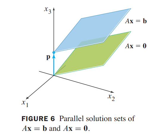
the solution set of $A\vec{x} = \vec{b}$ is a line through $\vec{p}$ parallel to the solution set of $A\vec{x} = \vec{0}$.
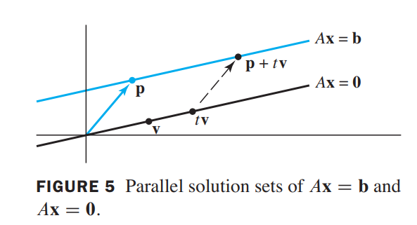
Figure 6 illustrates the case in which there are two free variables, the solution set is a plane, not a line.
Application of linear systems
Network Flow
💡For Example💡:
The network in Figure 2 shows the traffic flow (in vehicles per hour) over several one-way streets in downtown Baltimore during a typical early afternoon.
Determine the general flow pattern for the network.
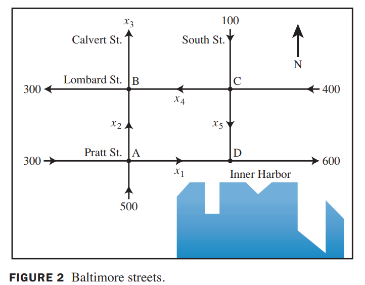
Solution:
| Intersection | Flow in | Flow out |
|---|---|---|
| A | 300+500 | = $x_1 + x2$ |
| B | $x_2 + x4$ | = 300 + $x_3$ |
| C | 100 + 400 | = $x_4 + x5$ |
| D | $x_1 + x5$ | = 600 |
$$
列方程,解方程如下:
\begin{matrix}
x_1 + x_2 = 800\\
x_2 - x_3 + x4 = 300\\
x_4 + x_5 = 500\\
x1 + x5 = 600\\
x_3 = 400
\end{matrix}
\sim
\begin{cases}
x_1 = 600 - x_5 \\
x_2 = 200 + x_5 \\
x_3 = 400 \\
x_4 = 500 - x_5\\
x_5 is free
\end{cases}
$$
Linear independence
线性相关(有非零解)和线性无关(只有零解)
An indexed set of vectors {${\vec{v_1}, \cdots, \vec{v_p}}$} in $R^n$ is said to be linearly independent if the vector equation
$$
x_1\vec{v_1} + x_2\vec{v_2} + \cdots + x_p\vec{v_p} = \vec{0}
$$
has only the trivial solution. The set {${\vec{v_1}, \cdots, \vec{v_p}}$} is said to be linealy dependent if there exist weights $c_1, \cdots, c_p$, not all zeros, such that
$$
c_1\vec{v_1} + c_2\vec{v_2} + \cdots + c_p\vec{v_p} = \vec{0}
$$
The columns of a matrix $A$ are linearly independent if and only if the equation $A\vec{x} = \vec{0}$has only the trivial solution,
当然可以通过观察发现两组向量是否线性相关,比如:
$$
\vec{v_1} = \begin{bmatrix}3\\1\end{bmatrix},\space
\vec{v_2} = \begin{bmatrix}6\\2\end{bmatrix}
\rightarrow
\vec{v_2} = 2\vec{v_1},
linear\space dependent
$$
A set of two vectors {$\vec{v_1},\vec{v_2}$} is linearly dependent if at least one of the vectors is a multiple of the other. The set is linearly independent if and only if neither of the vectors is a multiple of the other.
Sets of Two or More Vectors
如果至少能找到一个向量是其他向量的线性组合,那么这个向量集就是线性相关的
If a set contains more vectors than there are entries in each vector, then the set is linearly dependent. That is, any set {$\vec{v_1}, \cdots, \vec{v_p}$} in $R^n$ is linearly dependent if p > n
$$
n= 3, p = 5,
\overbrace{
\begin{bmatrix}* & * & * & * & * \\* & * & * & * & * \\* & * & * & * & * \\
\end{bmatrix}}^{p}
$$
$$
\begin{bmatrix}2\\1\end{bmatrix},\begin{bmatrix}4\\-1\end{bmatrix},\begin{bmatrix}-2\\2\end{bmatrix}
linearly-dependent, cause\space three\space vectors,
but\space two\space entries\space in \space each \space vector
$$
Introduction to Linear Transformation
In Computer Graphics, $A\vec{x}$ is not related to linear combination.
We think the matrix $A$ as an object that “acts” on a vector $\vec{v}$ by multiplication to produce a new vector called $A\vec{x}$.
Matrix Transformation
$$
\vec{x}\mapsto A\vec{x}
$$
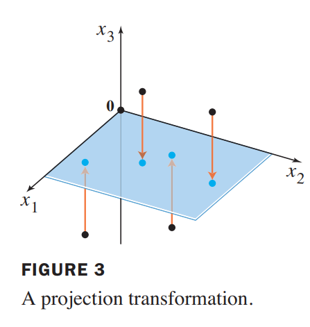
A projection transformation
if $A = \begin{bmatrix}
1 & 0 & 0\\
0 & 1 & 0 \\
0 & 0 & 0
\end{bmatrix}$, then the transformation $\vec{x}\mapsto A\vec{x}$ projects points in $R^3$ onto the $x_1x_2-plane$, because
$$
\begin{bmatrix}
x_1\\
x_2\\
x_3
\end{bmatrix}
\mapsto
\begin{bmatrix}
1 & 0 & 0\\
0 & 1 & 0 \\
0 & 0 & 0
\end{bmatrix}
\begin{bmatrix}
x_1\\
x_2\\
x_3
\end{bmatrix}
=
\begin{bmatrix}
x_1\\
x_2\\
0
\end{bmatrix}
$$
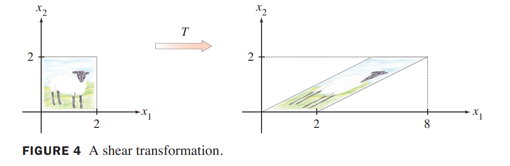
A shear transformation
if $A = \begin{bmatrix}
1 & 3 \\
0 & 1 \\
\end{bmatrix}$, the transformation $T:R^2\rightarrow R^2$ defined by $T(\vec{x}) = A\vec{x}$ is called shear transformation, because
$$
\begin{bmatrix}
0\\
2\\
\end{bmatrix}
\mapsto
\begin{bmatrix}
1 & 3 \\
0 & 1 \\
\end{bmatrix}
\begin{bmatrix}
0\\
2\\
\end{bmatrix}
=
\begin{bmatrix}
6\\
2
\end{bmatrix},
\begin{bmatrix}
2\\
2
\end{bmatrix}
\mapsto
\begin{bmatrix}
1 & 3 \\
0 & 1
\end{bmatrix}
\begin{bmatrix}
2\\
2
\end{bmatrix}
=
\begin{bmatrix}
8\\
2
\end{bmatrix}
$$
A transformation (or mapping) $T$ is linear if:
(i) $T(\vec{u} + \vec{v}) = T(\vec{u}) + T(\vec{v})$ for all $\vec{u},\vec{v}$ in the domain of $T$.
(ii) $T(c\vec{u}) = cT(\vec{u})$ for all scalars $c$ and all $\vec{u}$ in the domain of $T$.
Linear transformations preserve the operations of vector addition and scalar multiplication.
The Matrix of Linear Transformation
Let $T: R^n \rightarrow R^m$ be a linear transformation. Then there exists a unique matrix $A$ such that
$$
T(\vec{x}) = A\vec{x},for\space all\space x \space in R^n
$$
In fact, $A$ is the $m \times n$ matrix whose $j-th$ column is the vector $T(\vec{e_j})$, where $\vec{e_j}$ is the $j-th$ column of the identity matrix in $R^n$:
$$
A = \begin{bmatrix} T(\vec{e_1}) \cdots T(\vec{e_n})\end{bmatrix}\tag{3}
$$
the matrxi in (3) is called the standard matrix for the linear transformation T.
💡For example💡:
The columns of $I_2 = \begin{bmatrix}1 & 0 \\ 0 & 1\end{bmatrix}$ are $\vec{e_1} = \begin{bmatrix}1 \\ 0\end{bmatrix}$ and $\vec{e_2} = \begin{bmatrix}0 \\ 1\end{bmatrix}$. Suppose T is a linear transformation from $R^2$ into $R^3$ such that
$$
T(\vec{e_1}) = \begin{bmatrix}5 \\ -7 \\ 2\end{bmatrix}
and \space
T(\vec{e_2}) = \begin{bmatrix}-3 \\ 8 \\ 0\end{bmatrix}
$$
with no additional information, find a formula for the image of an arbitrary $\vec{x}$ in $R^2$
Solution:
$$
\vec{x} = \begin{bmatrix}x_1 \\ x_2 \end{bmatrix}
= x_1\begin{bmatrix}1 \\ 0\end{bmatrix} + x_2\begin{bmatrix}0 \\ 1\end{bmatrix}
= x_1\vec{e_1} + x_2\vec{e_2}
\\
T(\vec{x}) = x_1T(\vec{e_1}) + x_2T(\vec{e_2})
= \begin{bmatrix}5x_1 - 3x_2 \\ -7x_1+8x_2 \\ 2x_1+0\end{bmatrix}
\\
T(\vec{x}) = \begin{bmatrix}T(\vec{e_1}) & T(\vec{e_2})\end{bmatrix}\begin{bmatrix}x_1 \\ x_2\end{bmatrix}
= A\vec{x}
$$
A Rotation transformation
根据上文公式可以快速推导出2D旋转矩阵
$\begin{bmatrix}1 \\ 0\end{bmatrix}$ rotates into $\begin{bmatrix}\cos\psi \\ \sin\psi\end{bmatrix}$, and $\begin{bmatrix}0 \\ 1\end{bmatrix}$ rotates into $\begin{bmatrix}-\sin\psi \ \cos\psi\end{bmatrix}$
so the rotation matrix is $\begin{bmatrix}\cos\psi & -\sin\psi\\ \sin\psi & \cos\psi\end{bmatrix}$
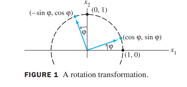
同理,其他如Reflection, expansion…变换都可以根据基向量进行推导
Let $T: R^n \rightarrow R^m$ be a linear transformation. Then $T$ is one-to-one if and only if the equation $T(\vec{x}) = \vec{0}$ has only the trivial solution.
Linear models in business,science, and engineering
Difference Equations(差分方程)
Several features of the system are each measured at discrete time intervals, producing a sequence of vectors $\vec{x_0},\vec{x_1},\vec{x_2},\cdots,\vec{x_k}$ The entries in $\vec{x_k}$ provide information about the state of the system at the time of the $k-th$ measurement.
If there is a matrix A such that $\vec{x_1} = A\vec{x_0}, \vec{x_2} = A\vec{x_1}$ and, in general,
$$
\vec{x_{k+1}} = A\vec{x_k}, k = 0,1,2,…\tag{5}
$$
then (5) is called a linear difference equation (or recurrence relation).
比如, 一个地区的人口增长可以用这种模型简单的表示
思考:矩阵快速幂怎么求?首先考虑普通的快速幂:
$$
\begin{aligned}
4 ^ {11} &= 4^{(1011)_2}\\
&= 4^{2^0}\cdot4^{2^1}\cdot4^{2^3}\\
4^{2^1} &= 4^{2^0} \cdot 4^{2^0}\\
4^{2^2} &= 4^{2^1} \cdot 4^{2^1}\\
4^{2^3} &= 4^{2^2} \cdot 4^{2^2}
\end{aligned}
$$
the c++ code is:
1 | //get a^k mod p |
接下来考虑矩阵快速幂:
💡for example💡: 如何快速计算Fibonacci的f(1000)?
$$
Fibonacci\\
f(0) = 0, f(1) = 1\\
f(n) = f(n-1) + f(n-2), n > 1
\\
建立矩阵方程如下:
let \space F(n) = \begin{bmatrix}f(n)\\f(n+1)\end{bmatrix}\\
AF(n) = F(n+1)\rightarrow
A\begin{bmatrix}f(n)\\ f(n+1)\end{bmatrix} =
\begin{bmatrix}f(n+1)\\ f(n+2)\end{bmatrix}
\rightarrow
A = \begin{bmatrix}0 & 1\\1 & 1\end{bmatrix}
\Rightarrow
F(n) = A^nF(0), F(0) = \begin{bmatrix}0\\1\end{bmatrix}
$$
1 | //get A^k * F_0 % p |

