Keywords: Conventional PCA, Probabilistic PCA, Nonlinear Latent Variable Models, Python
This is the Chapter12 ReadingNotes from book Bishop-Pattern-Recognition-and-Machine-Learning-2006. [Code_Python]
👉First Understanding PCA in Algebra >>
Principal Component Analysis
There are two commonly used definitions of PCA that give rise to the same algorithm: Maximum variance and Minimum-error.
Maximum variance formulation
$\pmb{x} \in R^D$, consider the projection onto a one-dimensional space (M = 1), We can define the direction of this space using a $D$-dimensional vector $\pmb{u_1}$, which for convenience (and without loss of generality) we shall choose to be a unit vector so that $\pmb{u_1^T u_1} = 1$.
the mean of samples
$$
\bar{\pmb{x}} = \frac{1}{N} \sum_{n=1}^N \pmb{x_n}
\tag{12.1}
$$
the variance of the projected data is given by
$$
\frac{1}{N} \sum_{n=1}^N \lbrace \pmb{u_1^Tx_n - u_1^T\bar{x}}\rbrace^2 = \pmb{u_1^TSu_1}
\tag{12.2}
$$
where $\pmb{S}$ is the data covariance matrix defined by
$$
\pmb{S} = \frac{1}{N} \sum_{n=1}^N (\pmb{x_n - \bar{x}})(\pmb{x_n - \bar{x}})^T
\tag{12.3}
$$
use Lagrange multiplier and make an unconstrained maximization of
$$
\pmb{u_1^TSu_1} + \lambda _1 (1 - pmb{u_1^Tu_1})
\tag{12.4}
$$
we get
$$
\pmb{Su_1} = \lambda _1 \pmb{u_1}
$$
so the variance will be a maximum when we set $\pmb{u_1}$ equal to the eigenvector having the largest eigenvalue $\lambda _1$. This eigenvector is known as the first principal component.
To summarize, principal component analysis involves evaluating the mean $\bar{\pmb{x}}$ and the covariance matrix $\pmb{S}$ of the data set and then finding the $M$ eigenvectors of S corresponding to the $M$ largest eigenvalues.
Minimum-error formulation
we introduce a complete orthonormal set of $D$-dimensional basis vectors $\lbrace \pmb{u_i} \rbrace$ where $i = 1, \cdots , D$ that satisfy
$$
\pmb{u_i^Tu_j} = \sigma_{ij}
\tag{12.7}
$$
Because this basis is complete, each data point can be represented exactly by a linear combination of the basis vectors
$$
\begin{aligned}
\pmb{x_n} &= \sum_{i=1}^D \alpha_{ni} \pmb{u_i} \\
&= \sum_{i=1}^D (\pmb{x_n^T u_i}) \pmb{u_i}
\end{aligned}
\tag{12.8}
$$
This simply corresponds to a rotation of the coordinate system to a new system defined by the $\lbrace \pmb{u_i} \rbrace$, and the original $D$ components $\lbrace x_{n1}, \cdots, x_{nD} \rbrace$ are replaced by an equivalent set $\lbrace \alpha_{n1}, \cdots, \alpha_{nD} \rbrace$.
The $M$ -dimensional linear subspace can be represented, without loss of generality, by the first $M$ of the basis vectors, and so we approximate each data point $\pmb{x_n}$ by
$$
\widetilde{\pmb{x_n}} = \sum_{i=1}^M z_{ni}\pmb{u_i} + \sum_{i = M+1}^{D} b_i \pmb{u_i}
\tag{12.10}
$$
we are going to minimize the distortion introduced by the reduction in dimensionality.
$$
J = \frac{1}{N} \sum_{n=1}^N ||\pmb{x_n - \widetilde{x_n}}||^2
\tag{12.11}
$$
get
$$
z_{nj} = \pmb{x_n^Tu_j}
\tag{12.12}
$$
$$
b_j = \bar{\pmb{x}}^T \pmb{u_j}
\tag{12.13}
$$
substitute (12.12), (12.13) to (12.11), we get
$$
\pmb{x_n - \widetilde{x_n}} = \sum_{i = M+1}^D \lbrace (\pmb{x_n - \bar{x}})^T \pmb{u_i}\rbrace \pmb{u_i}
\tag{12.14}
$$
from which we see that the displacement vector from $\pmb{x_n}$ to $\widetilde{\pmb{x_n}}$ lies in the space orthogonal to the principal subspace.
This result accords with our intuition that, in order to minimize the average squared projection distance, we should choose the principal component subspace to pass through the mean of the data points and to be aligned with the directions of maximum variance.
thus, we get distortion measure $J$ as
$$
J = \frac{1}{N} \sum_{n=1}^N \sum_{i=M+1}^D (\pmb{x_n^T u_i - \bar{x}^T u_i})^2 = \sum_{i=M+1}^D \pmb{u_i^T S u_i}
\tag{12.15}
$$
Applications of PCA
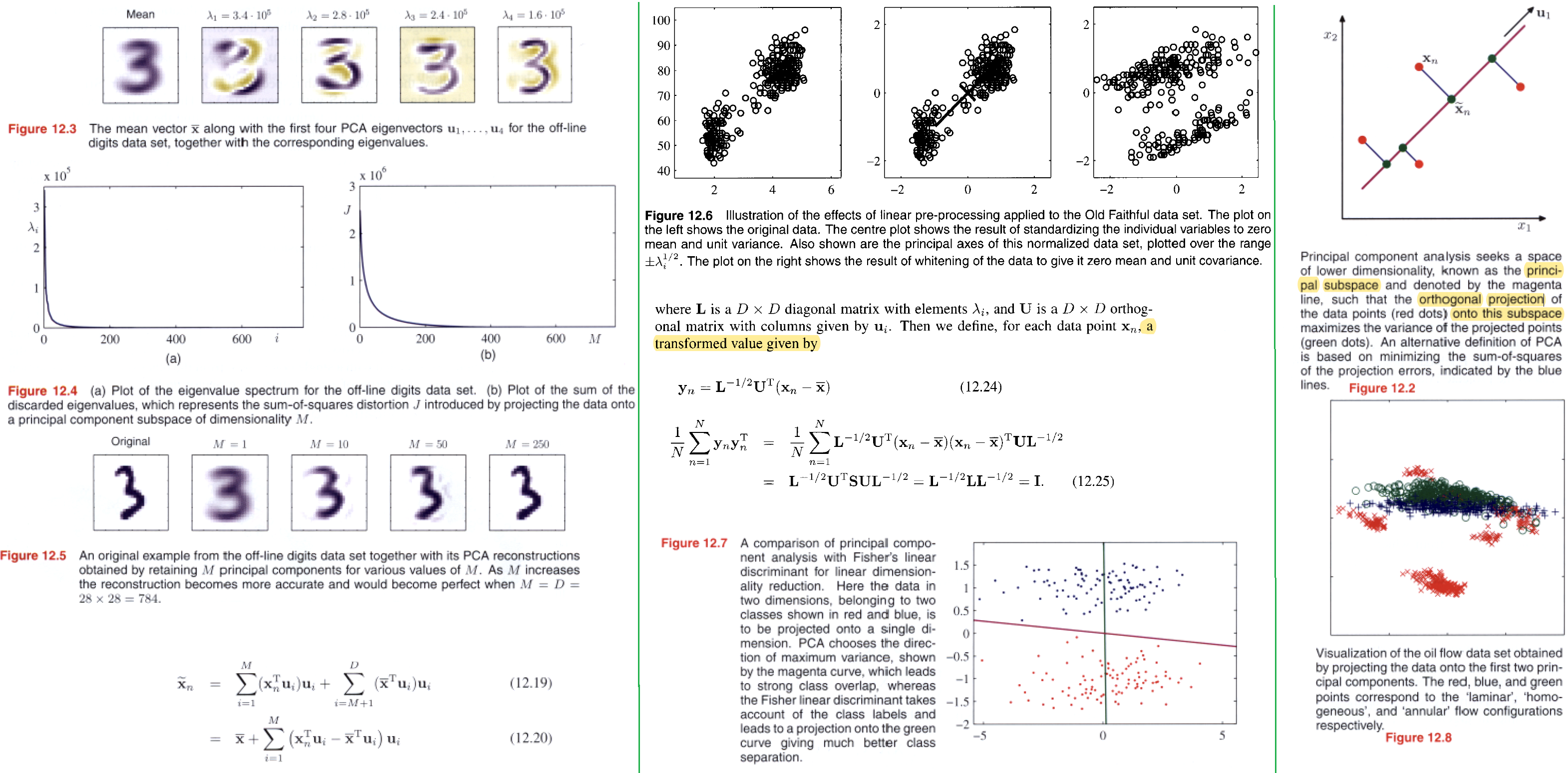
For data compression.
data pre-processing.
data visualization.
PCA for high-dimensional data
Probabilistic PCA
This reformulation of PCA, known as probabilistic peA, brings several advantages compared with conventional PCA.
- deal with missing values in the data set.
- trained using the EM algorithm, which is computationally efficient.
- forms the basis for a Bayesian treatment of PCA.
- can be used to model class-conditional densities.
- can be run generatively to provide samples from the distribution.
- represents a constrained form of the Gaussian distribution.
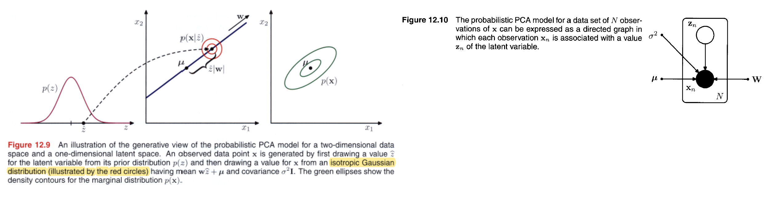
We can formulate probabilistic PCA by first introducing an explicit latent variable $\pmb{z}$ corresponding to the principal-component subspace.
the prior distribution is
$$
p(\pmb{z}) = N(\pmb{z | 0, I})
\tag{12.31}
$$
the conditional distribution is
$$
p(\pmb{x|z}) = N(\pmb{x}| \pmb{Wz + \mu}, \sigma^2 \pmb{I})
\tag{12.32}
$$
the columns of $\pmb{W}: D \times M$ span a linear subspace within the data space that corresponds to the principal subspace.
We can view the probabilistic PCA model from a generative viewpoint in which a sampled value of the observed variable is obtained by first choosing a value for the latent variable and then sampling the observed variable conditioned on this latent value. Specifically, the $D$-dimensional observed variable $\pmb{x}$ is defined by a linear transformation of the $M$-dimensional latent variable $\pmb{z}$ plus additive Gaussian ‘noise’, so that
$$
\pmb{x} = \pmb{Wz + \mu + \epsilon}
\tag{12.33}
$$
the marginal distribution of $p(\pmb{x})$ is
$$
p(\pmb{x}) = \int p(\pmb{x|z})p(\pmb{z}) d\pmb{z} = N(\pmb{x | \mu, C})
\tag{12.34}
$$
where the $D \times D$ matrix $\pmb{C}$ is
$$
\pmb{C} = \pmb{WW^T} + \sigma^2 \pmb{I}
\tag{12.36}
$$
from 👉2.116 >>, we get the posterior distribution $p(\pmb{z|x})$,
$$
p(\pmb{z|x}) = N(\pmb{z} | \pmb{M^{-1} W^T (x - \mu)}, \sigma^{2}\pmb{M})
\tag{12.42}
$$
where the $M \times M$ matrix $\pmb{M}$ is defined by
$$
\pmb{M} = \pmb{W^TW} + \sigma^2 \pmb{I}
$$
Maximum likelihood PCA
The corresponding log likelihood function is given by
$$
\begin{aligned}
\ln p(\pmb{X} | \pmb{\mu, W}, \sigma^2) &= \sum_{n=1}^N \ln p(\pmb{x_n} | \pmb{W, \mu}, \sigma^2) \\
&= -\frac{ND}{2} \ln(2\pi) - \frac{N}{2} \ln |\pmb{C}| - \frac{1}{2} \sum_{n=1}^N (\pmb{x_n - \mu})^T \pmb{C}^{-1} (\pmb{x_n - \mu}) \\
&= -\frac{N}{2} \lbrace D \ln(2\pi) + \ln |\pmb{C}| + Tr(\pmb{C^{-1}S})\rbrace
\end{aligned}
\tag{12.44}
$$
maximum log likelihood, we get
$$
\pmb{W_{ML}} = \pmb{U_{M}} (\pmb{L_M} - \sigma^2 \pmb{I})^{1/2} \pmb{R}
\tag{12.45}
$$
where, $\pmb{U_M}$ is a $D \times M$ matrix whose columns are given by any subset (of size $M$) of the eigenvectors of the data covariance matrix $\pmb{S}$, the $M \times M$ diagonal matrix $\pmb{L_M}$ has elements given by the corresponding eigenvalues $\lambda_i$, and $\pmb{R}$ is an arbitrary $M \times M$ orthogonal matrix.
$$
\sigma_{ML}^2 = \frac{1}{D - M} \sum_{i = M + 1}^D \lambda_i
\tag{12.46}
$$
so that $\sigma_{ML}^2$ is the average variance associated with the discarded dimensions.
Because $\pmb{R}$ is orthogonal, it can be interpreted as a rotation matrix in the $M \times M$ latent space. For the particular case of $\pmb{R} = \pmb{I}$, we see that the columns of $\pmb{W}$ are the principal component eigenvectors scaled by the variance parameters $\lambda_i - \sigma^2$.
The interpretation of these scaling factors is clear once we recognize that for a convolution of independent Gaussian distributions (in this case the latent space distribution and the noise model) the variances are additive.
Thus the variance $\lambda_i$ in the direction of an eigenvector $\pmb{u_i}$ is composed of the sum of a contribution $\lambda_i - \sigma^2$ from the projection of the unit-variance latent space distribution into data space through the corresponding column of $\pmb{W}$, plus an isotropic contribution of variance $\sigma^2$ which is added in all directions by the noise model.
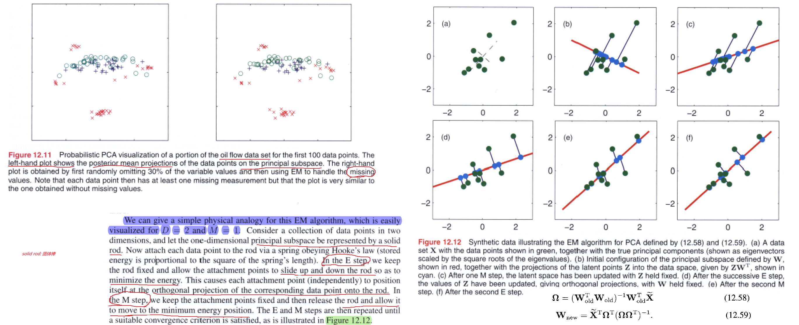
EM algorithm for PCA
In spaces of high dimensionality, there may be computational advantages in using an iterative EM procedure rather than working directly with the sample covariance matrix. This EM procedure can also be extended to the factor analysis model, for which there is no closed-form solution. Finally, it allows missing data to be handled in a principled way.
the complete-data log likelihood function takes the form
$$
\ln p(\pmb{X,Z} | \pmb{\mu, W}, \sigma^2) = \sum_{n=1}^N \lbrace \ln p(\pmb{x_n} | \pmb{z_n}) + \ln p(\pmb{z_n}) \rbrace
\tag{12.52}
$$
the $Q$ function(expectation of log likelihood function) is
$$
\begin{aligned}
E[\ln p(\pmb{X,Z} | \pmb{\mu, W}, \sigma^2)] &= -\sum_{n=1}^N \lbrace \frac{D}{2} \ln(2\pi\sigma^2) + \frac{1}{2} Tr(E[\pmb{z_nz_n^T}])\\
&+ \frac{1}{2\sigma^2} ||\pmb{x_n - \mu}||^2 - \frac{1}{\sigma^2} E[\pmb{z_n}]^T \pmb{W}^T (\pmb{x_n - \mu}) \\
&+ \frac{1}{2\sigma^2} Tr(E[\pmb{z_nz_n^T}] \pmb{W^TW})\rbrace
\end{aligned}
$$
where
$$
E[\pmb{z_n}] = \pmb{M^{-1}W^T(x_n - \bar{x})}
\tag{12.54}
$$
$$
E[\pmb{z_nz_n^T}] = \sigma^2 \pmb{M}^{-1} + E[\pmb{z_n}]E[\pmb{z_n}]^T
\tag{12.55}
$$
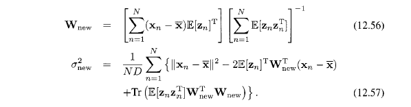
Now in the M step, we get
Note that this EM algorithm can be implemented in an on-line form in which each $D$-dimensional data point is read in and processed and then discarded before the next data point is considered.
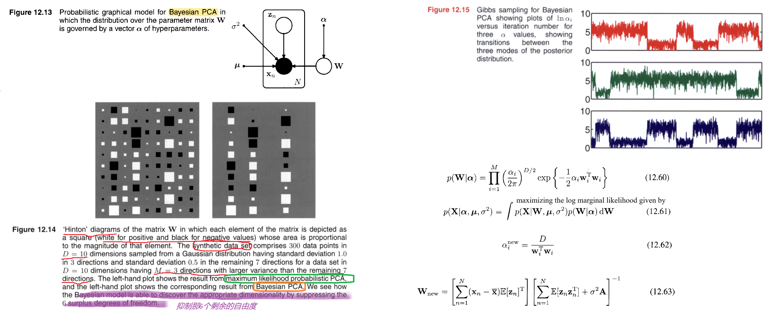
Bayesian PCA
We want to infer the reduced dimention $M$ by our model, not be given by users. So here comes Bayesian PCA, we use evidence approximation. Recall the definiton,
In Bayesian statistics, the evidence (also known as the marginal likelihood) is the probability of observing the data given a particular model, averaged over all possible parameter values. It serves as a normalizing constant when updating the prior beliefs to obtain the posterior distribution. The evidence is crucial for comparing different models and selecting the one that best explains the observed data.
The evidence for a model $M$ given the data $D$ is denoted as $p(D|M)$ and calculated as:
$$
p(D|M) = \int p(D|\theta, M) p(\theta|M) d\theta
$$
where
$p(D|\theta, M)$ is the likelihood, representing the probability of the data given the model parameters.
$p(\theta | M)$ is the prior, representing the prior distribution over the model parameters.
So here, we assume the prior of $\pmb{W}$ is Gaussian,
$$
p(\pmb{W} | \pmb{\alpha}) = \prod_{i=1}^M (\frac{\alpha_i}{2\pi})^{D/2} exp \lbrace -\frac{1}{2} \alpha_i \pmb{w_i^T w_i}\rbrace
\tag{12.60}
$$
The values of $\alpha_i$ are re-estimated during training by maximizing the log marginal likelihood given by
$$
p(\pmb{X}| \pmb{\alpha, \mu}, \sigma^2) = \int \underbrace{p(\pmb{X} | \pmb{W, \mu}, \sigma^2)}_{12.43} p(\pmb{W} | \pmb{\alpha}) d\pmb{W}
\tag{12.61}
$$
Because this integration is intractable, we make use of the Laplace approximation.
If we assume that the posterior distribution is sharply peaked, as will occur for sufficiently large data sets, then the re-estimation equations obtained by maximizing the marginal likelihood with respect to $\alpha_i$ take the simple form
$$
\alpha_i^{new} = \frac{D}{\pmb{w_i^Tw_i}}
\tag{12.62}
$$
which follows from 👉(3.98) >>,
These reestimations are interleaved with the EM algorithm updates for determining $\pmb{W}$ and $\sigma^2$, the only change is to the M. Step equation for $\pmb{W}$,
Factor analysis
Factor analysis is a linear-Gaussian latent variable model that is closely related to probabilistic PCA.
Kernel PCA
Kernel Principal Component Analysis (Kernel PCA) is an extension of the classical Principal Component Analysis (PCA) technique that allows for the nonlinear transformation of data by using kernel functions.
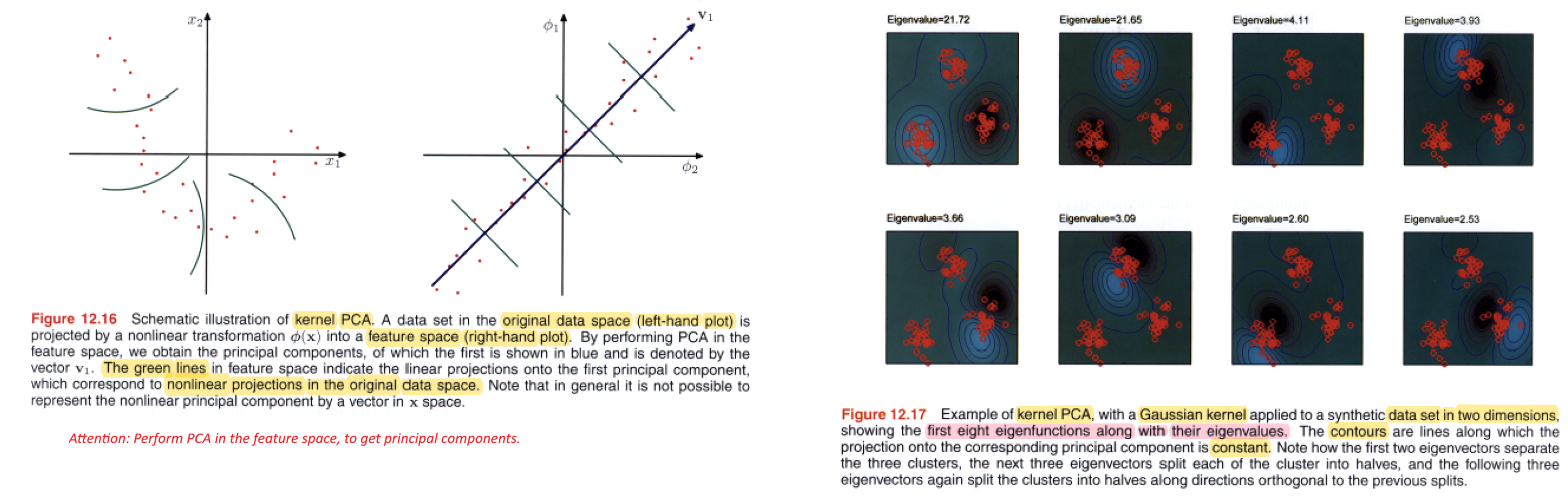
Kernel PCA is particularly useful for capturing complex, nonlinear relationships in the data. The choice of the kernel function and its parameters is crucial and may depend on the specific characteristics of the data.
Nonlinear Latent Variable Models
the issues of nonlinearity and non-Gaussianity are related because a general probability density can be obtained from a simple fixed reference density, such as a Gaussian, by making a nonlinear change of variables.
Independent component analysis
independent component analysis: the observed variables are related linearly to the latent variables, but for which the latent distribution is non-Gaussian.
Consider a situation in which two people are talking at the same time, and we record their voices using two microphones. If we ignore effects such as time delay and echoes, then the signals received by the microphones at any point in time will be given by linear combinations of the amplitudes of the two voices. The coefficients of this linear combination will be constant, and if we can infer their values from sample data, then we can invert the mixing process (assuming it is nonsingular) and thereby obtain two clean signals each of which contains the voice of just one person.
This type of problem is sometimes addressed using the following approach (MacKay, 2003) in which we ignore the temporal nature of the signals and treat the successive samples as i.i.d.
We consider a generative model in which there are two latent variables corresponding to the unobserved speech signal amplitudes, and there are two observed variables given by the signal values at the microphones.
The latent variables have a joint distribution that factorizes as,
$$
p(\pmb{z}) = \prod_{j=1}^M p(z_j)
\tag{12.89}
$$
and the observed variables are given by a linear combination of the latent variables.Given a data set of observations, The log likelihood can be maximized using gradient-based optimization giving rise to a particular version of independent component analysis.
The success of this approach requires that the latent variables have non-Gaussian distributions. Why?
- Recall that in probabilistic PCA (and in factor analysis) the latent-space distribution is given by a zero-mean isotropic Gaussian.
The model therefore cannot distinguish between two different choices for the latent variables where these differ simply by a rotation in latent space.
This can be verified directly by noting that the marginal density (12.35), and hence the likelihood function, is unchanged if we make the transformation $\pmb{W} \rightarrow \pmb{WR}$ where $\pmb{R}$ is an orthogonal matrix satisfying $\pmb{RR^T} = \pmb{I}$, because the matrix $\pmb{C}$ given by (12.36) is itself invariant.
$$
p(\pmb{x}) = N(\pmb{x | \mu, C})
\tag{12.35}
$$
$$
\pmb{C} = \pmb{WW^T} + \sigma^2 \pmb{I}
\tag{12.36}
$$- Another way to see why a Gaussian latent variable distribution in a linear model is insufficient to find independent components is to note that the principal components represent a rotation of the coordinate system in data space such as to diagonalize the covariance matrix, so that the data distribution in the new coordinates is then uncorrelated. Although zero correlation is a necessary condition for independence it is not, however, sufficient. In practice, a common choice for the latent-variable distribution is given by
$$
p(z_j) = \frac{1}{\pi \cosh(z_j)} = \frac{1}{\pi(e^{z_j} + e^{-z_j})}
\tag{12.90}
$$
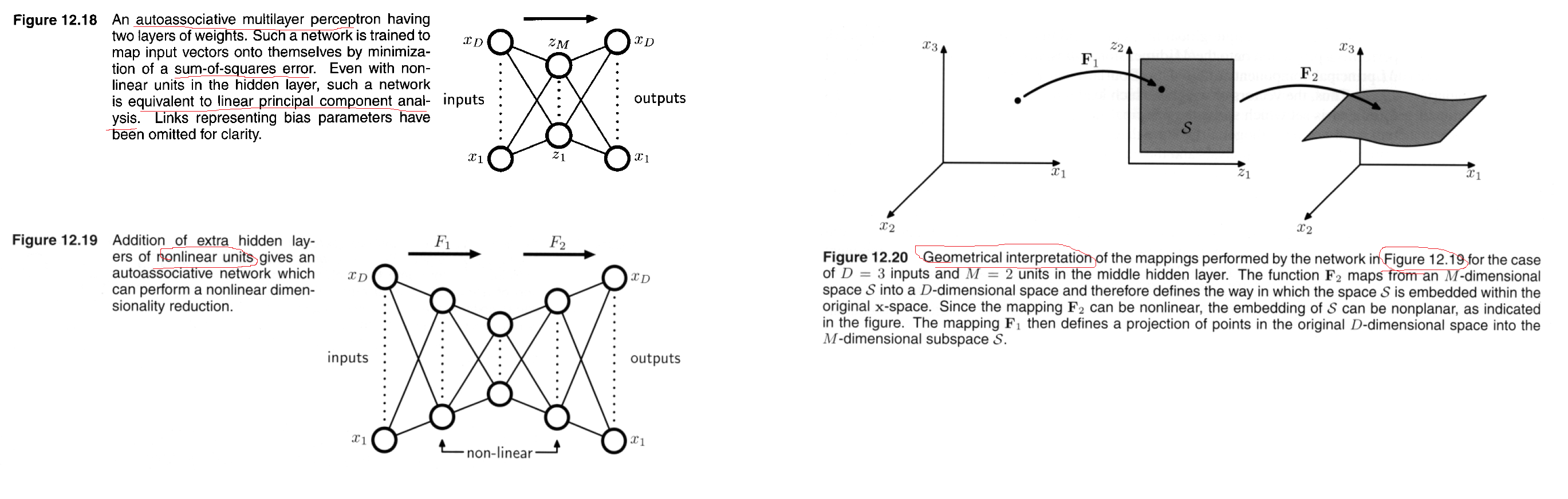
Autoassociative neural networks