Keywords: Hidden Markov Models, Python
This is the Chapter13 ReadingNotes from book Bishop-Pattern-Recognition-and-Machine-Learning-2006. [Code_Python]
Markov Models
we can use the product rule to express the joint distribution for a sequence of observations in the form
$$
p(\pmb{x_1}, \cdots, \pmb{x_N}) = \prod_{n=1}^N p(\pmb{x_n} | \pmb{x_1}, \cdots, \pmb{x_{n-1}})
\tag{13.1}
$$
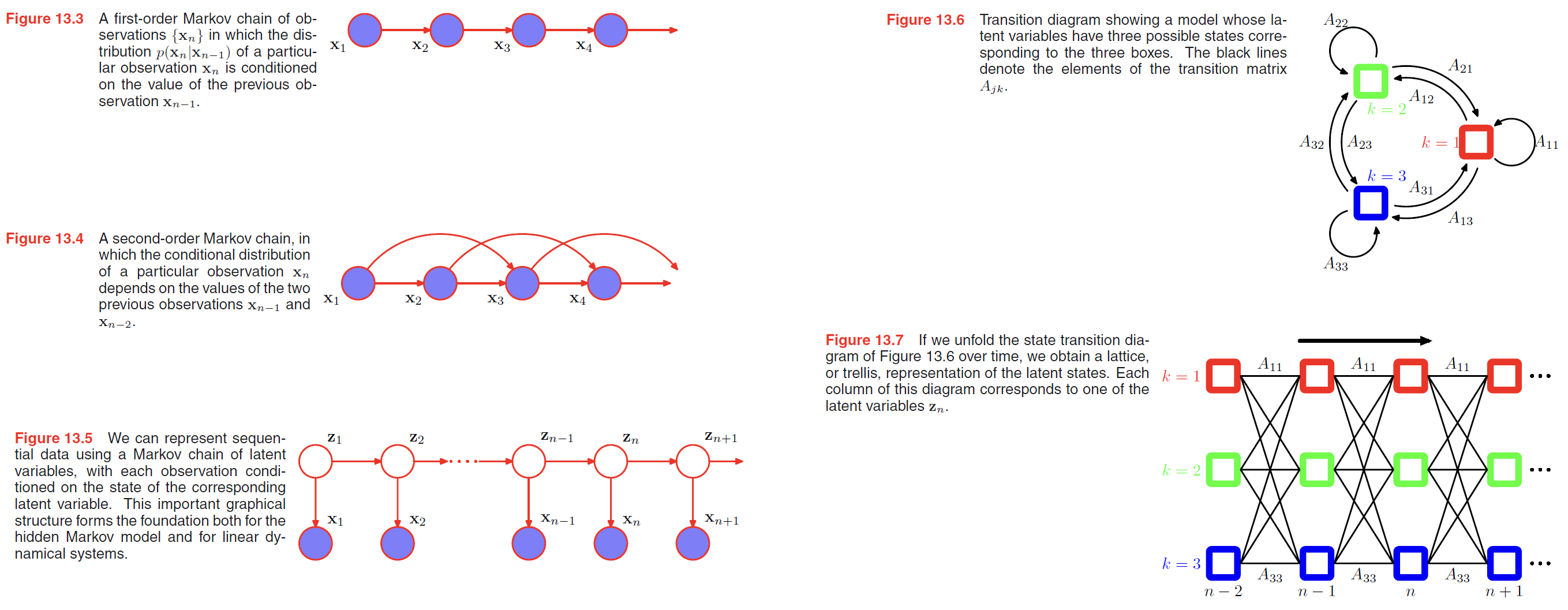
the joint distribution for a sequence of observations under first-order Markov chain in the form
$$
p(\pmb{x_1}, \cdots, \pmb{x_N}) = p(\pmb{x_1}) \prod_{n=2}^N p(\pmb{x_n} | \pmb{x_{n-1}})
\tag{13.2}
$$
the joint distribution for a sequence of observations under second-order Markov chain in the form
$$
p(\pmb{x_1}, \cdots, \pmb{x_N}) = p(\pmb{x_1}) p(\pmb{x_2} | \pmb{x_1}) \prod_{n=3}^N p(\pmb{x_n} | \pmb{x_{n-1}}, \pmb{x_{n-2}})
\tag{13.4}
$$
The joint distribution for Hidden Markov Model or linear dynamical system is given by
$$
p(\pmb{x_1}, \cdots, \pmb{x_N}, \pmb{z_1}, \cdots, \pmb{z_N}) = p(\pmb{z_1}) [\prod_{n=2}^N p(\pmb{z_n | z_{n-1}})] \prod_{n=1}^N p(\pmb{x_n | z_n})
\tag{13.6}
$$
Hidden Markov Models
HMM can also be interpreted as an extension of a mixture model in which the choice of mixture component for each observation is not selected independently but depends on the choice of component for the previous observation.
the conditional distribution of latent variable is
$$
p(\pmb{z_n} | \pmb{z_{n-1}}, \pmb{A}) = \prod_{k=1}^K prod_{j=1}^K A_{jk}^{z_{n-1,j} z_{nk}}
\tag{13.7}
$$
Because the latent variables are $K$-dimensional binary variables, this conditional distribution corresponds to a table of numbers that we denote by $\pmb{A}$, the elements of which are known as transition probabilities.
The initial latent node $\pmb{z_1}$ is special in that it does not have a parent node
$$
p(\pmb{z_1} | \pmb{\pi}) = \prod_{k=1}^K \pi_k^{z_1k}
\tag{13.8}
$$
where, $\sum_k \pi_k = 1$
the emission probabilities in the form
$$
p(\pmb{x_n} | \pmb{z_n}, \pmb{\phi}) = \prod_{k=1}^K p(\pmb{x_n} | \phi_k )^{z_{nk}}
\tag{13.9}
$$
The joint probability distribution over both latent and observed variables is then given by
$$
p(\pmb{X,Z} | \pmb{\theta}) = p(\pmb{z_1} | \pmb{\pi}) [\prod_{n=1}^N p(\pmb{z_n} | \pmb{z_{n-1}}, \pmb{A})] \prod_{m=1}^N \underbrace{p(\pmb{x_m} | \pmb{z_m}, \pmb{\phi})}_{emission-probabilities}
\tag{13.10}
$$
where, $\pmb{X} = \lbrace \pmb{x_1}, \cdots, \pmb{x_N}\rbrace$, $\pmb{Z} = \lbrace \pmb{z_1}, \cdots, \pmb{z_N}\rbrace$, and $\pmb{\theta} = \lbrace \pmb{\pi, A, \phi}\rbrace$ denotes the set of parameters governing the model.
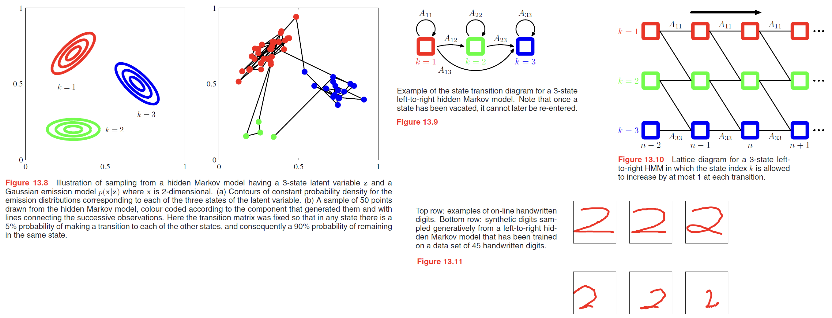
Many applications of hidden Markov models, for example speech recognition, or on-line character recognition, make use of left-to-right architectures. As an illustration of the left-to-right hidden Markov model, we consider an example involving handwritten digits.
Here we train a hidden Markov model on a subset of data comprising 45 examples of the digit ‘2’. There are $K = 16$ states, each of which can generate a line segment of fixed length having one of 16 possible angles, and so the emission distribution is simply a $16 \times 16$ table of probabilities associated with the allowed angle values for each state index value. Transition probabilities are all set to zero except for those that keep the state index $k$ the same or that increment it by 1, and the model parameters are optimized using 25 iterations of EM. We can gain some insight into the resulting model by running it generatively, as shown in Figure 13.11.
Maximum likelihood for the HMM
If we have observed a data set $\pmb{X} = \lbrace \pmb{x_1}, \cdots, \pmb{x_N} \rbrace$, we can determine the parameters of an HMM using maximum likelihood.
The likelihood function is obtained from the joint distribution (13.10) by marginalizing over the latent variables
$$
p(\pmb{X} | \pmb{\theta}) = \sum_{\pmb{Z}} p(\pmb{X, Z} | \pmb{\theta})
\tag{13.11}
$$
Direct maximization of the likelihood function will therefore lead to complex expressions with no closed-form solutions, as was the case for simple mixture models(recall that a mixture model for i.i.d. data is a special case of the HMM). We therefore turn to the expectation maximization algorithm to find an efficient framework for maximizing the likelihood function in hidden Markov models—EM Algorithm.
EM Algorithm for HMM is now as follows:
- choose an initial value $\pmb{\theta}^{old}$ for the model parameters.
- E. Step:
take these parameter values and find the posterior distribution of the latent variables
$$
p(\pmb{Z}|\pmb{X}, \pmb{\theta}^{old})
$$
use this posterior distribution to evaluate the expectation of the logarithm of the complete-data likelihood function
$$
Q(\pmb{\theta, \theta^{old}}) = \sum_{Z} p(\pmb{Z}|\pmb{X}, \pmb{\theta}^{old}) \ln p(\pmb{X,Z} | \pmb{\theta})
\tag{13.12}
$$
here, We shall use $\gamma(\pmb{z_n})$ to denote the marginal posterior distribution of a latent variable zn, and $\xi(\pmb{z_{n−1}}, \pmb{z_n})$ to denote the joint posterior distribution of two successive latent variables, so that
$$
\gamma(\pmb{z_n}) = p(\pmb{z_n} | \pmb{X}, \pmb{\theta}^{old})
\tag{13.13}
$$
$$
\xi(\pmb{z_{n-1}, z_n}) = p(\pmb{z_{n-1}, z_n} | \pmb{X}, \pmb{\theta}^{old})
\tag{13.14}
$$
Because the expectation of a binary random variable is just the probability that it takes the value 1, we have
$$
\gamma(z_{nk}) = E[z_{nk}] = \sum_{\pmb{z}} \gamma(\pmb{z}) z_{nk}
\tag{13.15}
$$
$$
\xi(z_{n-1,j}, z_{nk}) = E[z_{n-1,j}, z_{nk}] = \sum_{\pmb{z}} \gamma(\pmb{z})z_{n-1,j}, z_{nk}
\tag{13.16}
$$
thus,
$$
Q(\pmb{\theta, \theta^{old}}) = \sum_{k=1}^K \gamma(z_{1k}) \ln \pi_k + \sum_{n=2}^N \sum_{j=1}^K \sum_{k=1}^K \xi(z_{n-1,j}, z_{nk}) \ln A_{jk} + \sum_{n=1}^N \sum_{k=1}^K \gamma(z_{nk}) \ln p(\pmb{x_n}|\pmb{\phi_k})
\tag{13.17}
$$ - M. Step:
maximize the function $Q(\pmb{\theta}, \pmb{\theta}^{old})$ with respect to $\pmb{\theta} = \lbrace \pmb{\pi, A, \phi} \rbrace$ in which we treat $\gamma(\pmb{z_n})$ and $p(\pmb{z_{n-1}, z_n} | \pmb{X}, \pmb{\theta}^{old})$ as constant.
3.1. Maximization with respect to $\pmb{π}$ and $\pmb{A}$ is easily achieved using appropriate Lagrange multipliers with the results
$$
\pi_k = \frac{\gamma(z_{1k})}{\sum_{j=1}^K \gamma(z_{1j})}
\tag{13.18}
$$
$$
A_{jk} = \frac{\sum_{n=2}^N \xi(z_{n-1,j}, z_{nk})}{\sum_{l=1}^K \sum_{n=2}^N \xi(z_{n-1,j}, z_{nl})}
\tag{13.19}
$$
3.2. maximize the function with respect to $\phi_k$, suppose Gaussian emission densities we have $p(\pmb{x}|\phi_k) = N(\pmb{x} | \pmb{\mu_k}, \pmb{\Sigma_k})$
$$
\pmb{\mu_k} = \frac{\sum_{n=1}^N \gamma(z_{nk})\pmb{x_n}}{\sum_{n=1}^N \gamma(z_{nk})}
\tag{13.20}
$$
$$
\pmb{\Sigma_k} = \frac{\sum_{n=1}^N \gamma(z_{nk})(\pmb{x_n - \mu_k})(\pmb{x_n - \mu_k})^T}{\sum_{n=1}^N \gamma(z_{nk})}
\tag{13.21}
$$
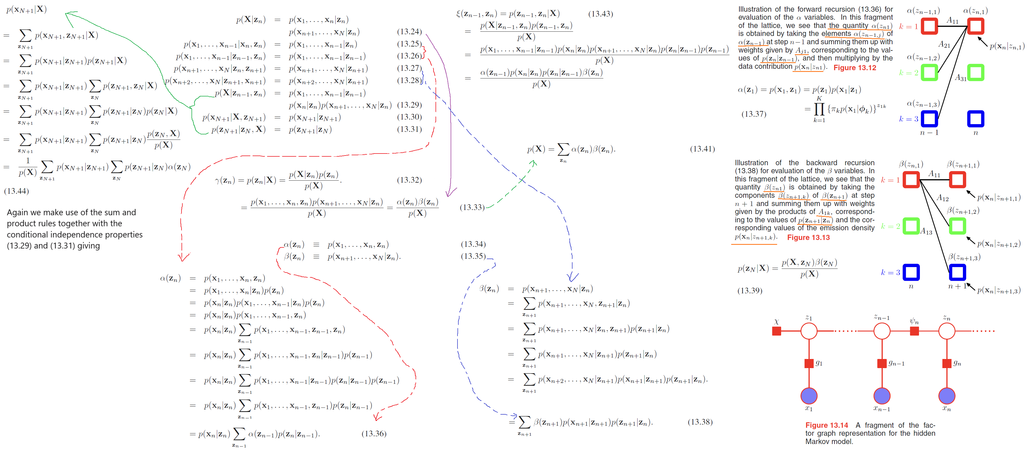
The forward-backward algorithm
Next we seek an efficient procedure for evaluating the quantities $\gamma(z_{nk})$ and $\xi(z_{n-1,j}, z_{nk})$, corresponding to the E step of the EM algorithm.
Here, we use alpha-beta algorithm, which is a variant of forward-backward algorithm or Baum-Welch algorithm.
Let us summarize the steps required to train a hidden Markov model using the EM algorithm.
- make an initial selection of the parameters $\pmb{\theta}^{old}$, where $\pmb{\theta} = (\pmb{\pi, A, \phi})$.
1.1. The $\pmb{A}$ and $\pmb{\pi}$ parameters are often initialized either uniformly or randomly from a uniform distribution (respecting their non-negativity and summation constraints).
1.2. Initialization of the parameters $\pmb{\phi}$ will depend on the form of the distribution.
For instance in the case of Gaussians, the parameters $\pmb{\mu_k}$ might be initialized by applying the $K$-means algorithm to the data, and $\pmb{\Sigma_k}$ might be initialized to the covariance matrix of the corresponding $K$ means cluster.
1.3. Run both the forward $\alpha$ recursion and the backward $\beta$ recursion and use the results to evaluate $\gamma(\pmb{z_n})$ and $\xi(\pmb{z_{n−1}}, \pmb{z_n})$. - M.Step in last Section.
- We then continue to alternate between E and M steps until some convergence criterion is satisfied, for instance when the change in the likelihood function is below some threshold.

