Keywords: Boosting, Conditional Mixture Models(linear regression, logistic regression), EM Algorithm
This is the Chapter14 ReadingNotes from book Bishop-Pattern-Recognition-and-Machine-Learning-2006.
Bayesian Model Averaging
Difference between Bayesian Model Averaging and Model Combination Methods.
- in Bayesian model averaging, the whole data set is generated by a single model(e.g. this single model is a mixture of Gaussians).
$$
p(X) = \sum_{h=1}^H p(\pmb{X} | h) p(h)
\tag{14.6}
$$
The interpretation of this summation over $h$ is that just one model is responsible for generating the whole data set, and the probability distribution over $h$ simply reflects our uncertainty as to which model that is.
As the size of the data set increases, this uncertainty reduces, and the posterior probabilities $p(h|\pmb{X})$ become increasingly focussed on just one of the models.
- Model Combination methods, e.g. mixture of Gaussians
$$
p(\pmb{x}) = \sum_{k=1}^K \pi_k N(\pmb{x} | \pmb{\mu_k}, \Sigma_k)
$$
$$
p(\pmb{X}) = \prod_{n=1}^N p(\pmb{x_n}) = \prod_{n=1}^N [\sum_{z_n} p(\pmb{x_n}, \pmb{z_n})]
\tag{14.5}
$$
The model contains a binary latent variable $\pmb{z}$ that indicates which component of the mixture is responsible for generating the corresponding data point.
Committees
For instance, we might train $L$ different models and then make predictions using the average of the predictions made by each model. Such combinations of models are sometimes called committees.
Why we need committees?
Recall the 👉Bias-Variance Decomposition >> in Section 3.
Such a procedure can be motivated from a frequentist perspective by considering the trade-off between bias and variance, which decomposes the error due to a model into the bias component that arises from differences between the model and the true function to be predicted, and the variance component that represents the sensitivity of the model to the individual data points.
when we trained multiple polynomials using the sinusoidal data, and then averaged the resulting functions, the contribution arising from the variance term tended to cancel, leading to improved predictions. When we averaged a set of low-bias models (corresponding to higher order polynomials), we obtained accurate predictions for the underlying sinusoidal function from which the data were generated.
But this “average method” has been proven not good enough, in order to achieve more significant improvements, we turn to a more sophisticated technique for building committees, known as boosting.
Boosting
The principal difference between boosting and the committee methods such as bagging discussed above, is that the base classifiers are trained in sequence, and each base classifier is trained using a weighted form of the data set in which the weighting coefficient associated with each data point depends on the performance of the previous classifiers.
In particular, points that are misclassified by one of the base classifiers are given greater weight when used to train the next classifier in the sequence. Once all the classifiers have been trained, their predictions are then combined through a weighted majority voting scheme, as illustrated schematically in Figure 14.1.
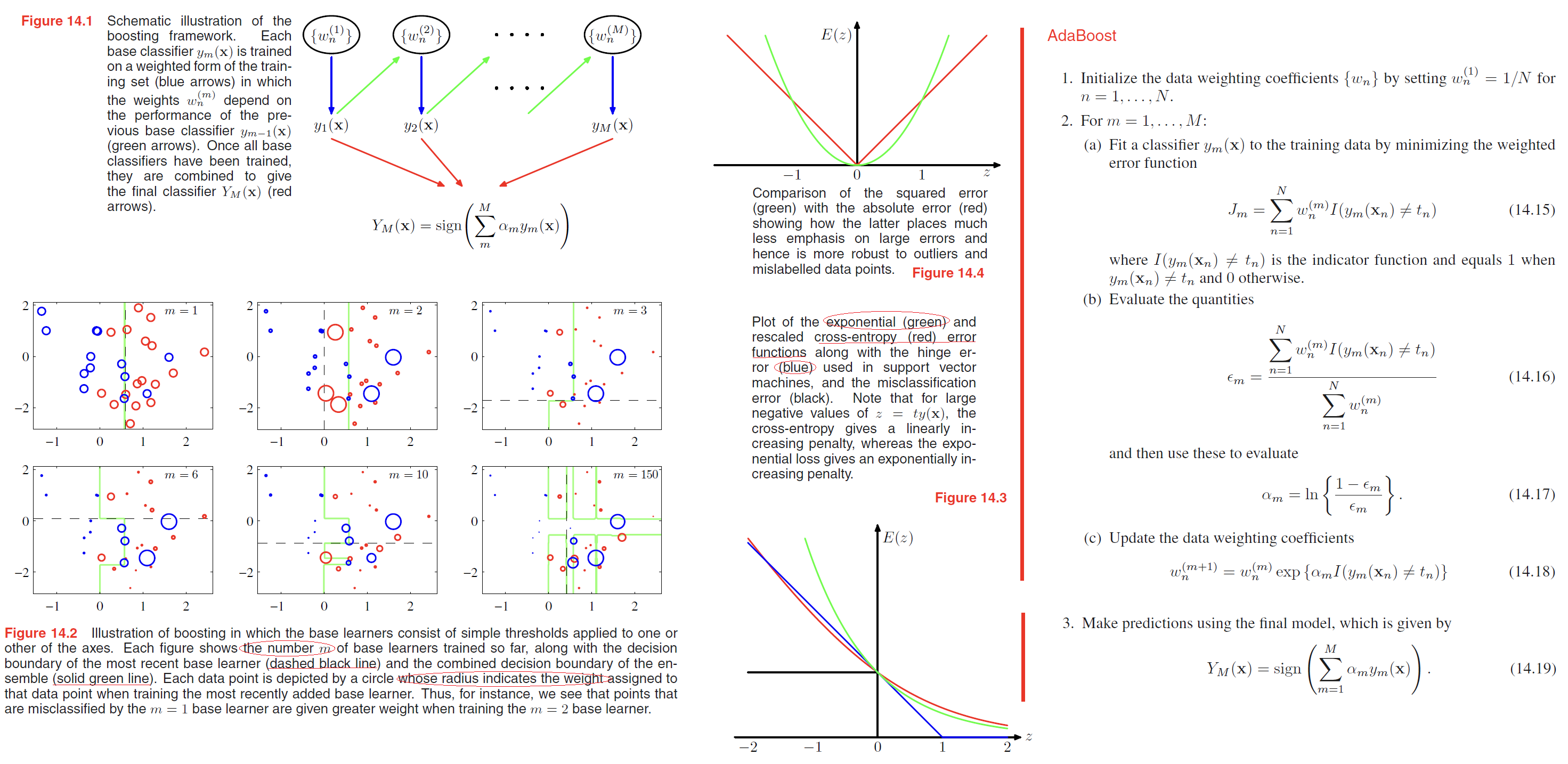
Minimizing exponential error
Friedman et al. (2000) gave a different and very simple interpretation of boosting in terms of the sequential minimization of an exponential error function.
Consider the exponential error function defined by
$$
E = \sum_{n=1}^N exp \lbrace -t_n f_m(\pmb{x_n})\rbrace
\tag{14.20}
$$
where
$$
f_m(\pmb{x}) = \frac{1}{2} \sum_{l=1}^m a_l y_l(\pmb{x})
\tag{14.21}
$$
Our goal is to minimize $E$ with respect to both the weighting coefficients $\alpha_l$ and the parameters of the base classifiers $y_l(\pmb{x})$.
we shall suppose that the base classifiers $y_1(x), \cdots , y_{m−1}(x)$ are fixed, as are their coefficients $\alpha_1, \cdots , \alpha_{m-1}$, and so we are minimizing only with respect to $\alpha_m$ and $y_m(x)$.
$$
\begin{aligned}
E &= \sum_{n=1}^N exp \lbrace -t_nf_{m-1}(\pmb{x_n}) - \frac{1}{2} t_n \alpha_m y_m(\pmb{x_n})\rbrace \\
&= \sum_{n=1}^N w_n^{m} exp \lbrace - \frac{1}{2} t_n \alpha_m y_m(\pmb{x_n})\rbrace
\end{aligned}
\tag{14.22}
$$
where
$$
w_n^{m} = exp \lbrace -t_nf_{m-1}(\pmb{x_n}) \rbrace
$$
can be viewed as constants because we are optimizing only $\alpha_m$ and $y_m(x)$.
If we denote by $T_m$ the set of data points that are correctly classified by $y_m(\pmb{x})$, and if we denote the remaining misclassified points by $M_m$, then we can in turn rewrite the error function in the form
…
Anyway, the formula following just proves that the AdaBoost method is a sequential minimization of exp error.
Error functions for boosting
Tree-based Models
For any new input x, we determine which region it falls into by starting at the top of the tree at the root node and following a path down to a specific leaf node according to the decision criteria at each node. Note that such decision trees are not probabilistic graphical models. Within each region, there is a separate model to predict the target variable.
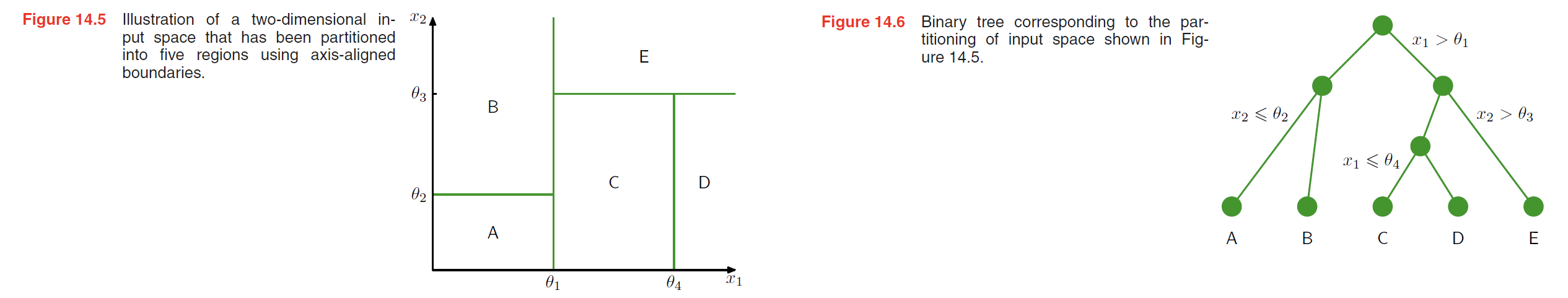
Consider first a regression problem in which the goal is to predict a single target variable $t$ from a $D$-dimensional vector $\pmb{x} = (x_1, \cdots , x_D)^T$ of input variables. The training data consists of input vectors {\pmb{x_1}, \cdots , \pmb{x_N}} along with the corresponding continuous labels ${t_1, \cdots , t_N}$.
If the partitioning of the input space is given, and we minimize the sum-of-squares error function, then the optimal value of the predictive variable within any given region is just given by the average of the values of tn for those data points that fall in that region.
…
However, in practice it is found that the particular tree structure that is learned is very sensitive to the details of the data set, so that a small change to the training data can result in a very different set of splits (Hastie et al., 2001).
Conditional Mixture Models
Mixtures of linear regression models
Here we consider a simple example corresponding to a mixture of linear regression models, which represents a straightforward extension of the Gaussian mixture model discussed in Section 9.2 to the case of conditional Gaussian distributions.
- the mixture distribution (conditional Gaussian distributions) can be written as
$$
p(\pmb{t} | \pmb{\theta}) = \sum_{k=1}^K \pi_k N(t | \pmb{w_k}^T\pmb{\phi}, \beta^{-1})
\tag{14.34}
$$ - The log likelihood function for this model, given a data set of observations $\lbrace \phi_n, t_n\rbrace$ takes the form
$$
\ln p(\pmb{t} | \pmb{\theta}) = \sum_{n=1}^N \ln (\sum_{k=1}^K \pi_k N(t_n | \pmb{w_k}^T \phi_n, \beta^{-1}))
\tag{14.35}
$$ - The complete-data log likelihood function then takes the form
$$
\ln p(\pmb{t, Z} | \pmb{\theta}) = \sum_{n=1}^N \sum_{k=1}^K z_{nk}\ln \lbrace \pi_k N(t_n | \pmb{w_k}^T \phi_n, \beta^{-1}) \rbrace
$$
EM Algorithm for this formula is now as follows:
choose an initial value $\pmb{\theta}^{old}$ for the model parameters.
E. Step:
use current $\pmb{\theta}$ to evaluate the posterior probabilities, or responsibilities, of each component $k$ for every data point $n$ given by
$$
\begin{aligned}
\gamma_{nk} &= E[z_{nk}]\\
&= p(k | \phi_n, \pmb{\theta}^{old})\\
&= \frac{\pi_k N(t_n | \pmb{w_k}^T\phi_n, \beta^{-1})}{\sum_j \pi_j N(t_n | \pmb{w_j}^T\phi_n, \beta^{-1})}
\end{aligned}
\tag{14.37}
$$
use current responsibilities to determine the expectation, with respect to the posterior distribution $p(\pmb{Z}|\pmb{t}, \pmb{\theta}^{old})$, of the complete-data log likelihood
$$
\begin{aligned}
Q(\pmb{\theta}, \pmb{\theta}^{old}) &= E_{\pmb{Z}}[\ln p(\pmb{t, Z} | \pmb{\theta})]\\
&= \sum_{n=1}^N \sum_{k=1}^K \gamma_{nk} \lbrace \ln \pi_k + \ln N(t_n | \pmb{w_k}^T \phi_n, \beta^{-1})\rbrace
\end{aligned}
\tag{14.37}
$$M. Step:
3.1. maximize the function $Q(\pmb{\theta}, \pmb{\theta}^{old})$ with respect to $\pi_k$
$$
\pi_k = \frac{1}{N} \sum_{n=1}^{N} \gamma_{nk}
\tag{14.38}
$$
3.2. maximization with respect to the parameter vector $\pmb{w_k}$ of the $k$ th linear regression model
$$
Q(\pmb{\theta}, \pmb{\theta}^{old}) = \sum_{n=1}^N \gamma_{nk} \lbrace -\frac{\beta}{2} (t_n - \pmb{w_k}^T\phi_n)^2 \rbrace + const
\tag{14.39}
$$
where the constant term includes the contributions from other weight vectors $\pmb{w_j}$ for $j \neq k$.
Setting the derivative of (14.39) with respect to wk equal to zero gives
$$
\begin{aligned}
0 &= \sum_{n=1}^N \gamma_{nk}(t_n - \pmb{w_k}^T\phi_n)\phi_n\\
&= \pmb{\Phi^T R_k (t - \Phi w_k)}
\end{aligned}
\tag{14.40}
$$
where
$$
\pmb{R_k} = diag(\gamma_{nk})
$$
solving for $\pmb{w_k}$, we get
$$
\pmb{w_k} = (\pmb{\Phi^T R_k \Phi})^{-1} \pmb{\Phi^T R_k t}
\tag{14.42}
$$
This represents a set of modified normal equations corresponding to the weighted least squares problem, of the same form as (4.99) found in the context of logistic regression.
$$
\pmb{w}^{(new)} = \pmb{(\Phi^T R \Phi)^{-1} \Phi^T R z}
\tag{4.99}
$$
👉iterative reweighted least squares,IRLS >>3.3. maximization with respect to the $\beta$
$$
Q(\pmb{\theta}, \pmb{\theta}^{old}) = \sum_{n=1}^N \sum_{k=1}^K \gamma_{nk} \lbrace \frac{1}{2} \ln \beta - \frac{\beta}{2}(t_n - \pmb{w_k}^T \phi_n)^2 \rbrace
\tag{14.43}
$$
Setting the derivative with respect to $\beta$ equal to zero,
$$
\frac{1}{\beta} = \frac{1}{N} \sum_{n=1}^N \sum_{k=1}^K \gamma_{nk} (t_n - \pmb{w_k}^T \phi_n)^2
\tag{14.44}
$$
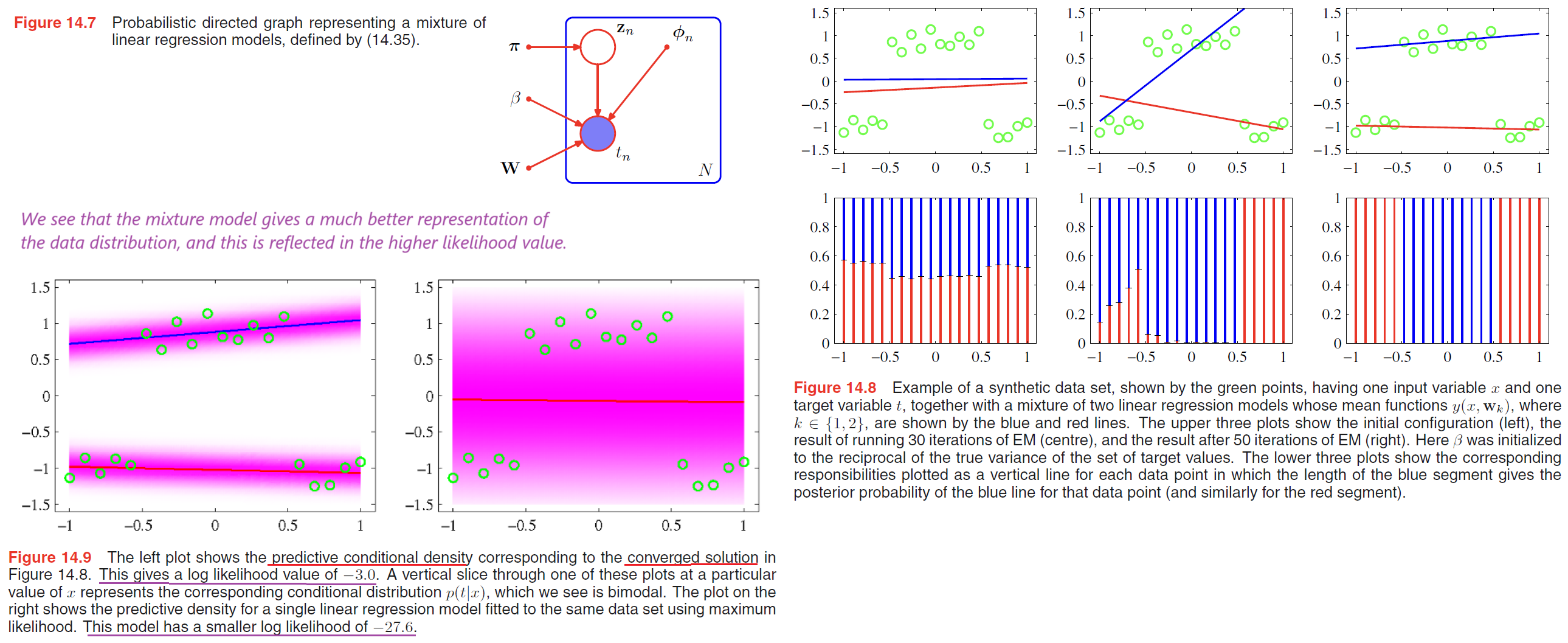
However, the mixture model also assigns significant probability mass to regions where there is no data because its predictive distribution is bimodal for all values of $x$. This problem can be resolved by extending the model to allow the mixture coefficients themselves to be functions of $x$, leading to models such as the mixture density networks discussed in Section 5.6, and hierarchical mixture of experts discussed in Section 14.5.3
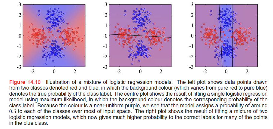
Mixtures of logistic models
The conditional distribution of the target variable, for a probabilistic mixture of $K$ logistic regression models, is given by
$$
p(t | \phi, \pmb{\theta}) = \sum_{k=1}^K \pi_k y_k^t [1 - y_k]^{1-t}
\tag{14.45}
$$corresponding likelihood function is then given by
$$
p(\pmb{t} | \pmb{\theta}) = \prod_{n=1}^N (\sum_{k=1}^K \pi_k y_{nk}^{t_n} [1 - y_{nk}]^{1 - t_n})
\tag{14.46}
$$complete-data likelihood function is then given by
$$
p(\pmb{t, Z} | \pmb{\theta}) = \prod_{n=1}^N \prod_{k=1}^K \lbrace \pi_k y_{nk}^{t_n} [1-y_{nk}]^{1-t_n} \rbrace ^{z_{nk}}
\tag{14.47}
$$
where $\pmb{Z}$ is the matrix of latent variables with elements $z_{nk}$.E. Step
$$
\begin{aligned}
\gamma_{nk} &= E[z_{nk}]\\
&= p(k | \phi_n, \pmb{\theta}^{old})\\
&= \frac{\pi_k y_{nk}^{t_n} [1 - y_{nk}]^{1 - t_n}}{\sum_j \pi_j y_{nj}^{t_n} [1 - y_{nj}]^{1 - t_n}}
\end{aligned}
\tag{14.48}
$$
$$
\begin{aligned}
Q(\pmb{\theta}, \pmb{\theta}^{old}) &= E_{\pmb{Z}}[\ln p(\pmb{t, Z} | \pmb{\theta})]\\
&= \sum_{n=1}^N \sum_{k=1}^K \gamma_{nk} \lbrace \ln \pi_k + t_n \ln y_{nk} + (1-t_n) \ln(1-y_{nk})\rbrace
\end{aligned}
\tag{14.49}
$$M. Step
$$
\pi_k = \frac{1}{N} \sum_{n=1}^N \gamma_{nk}
\tag{14.50}
$$
Note that the M step does not have a closed-form solution and must be solved iteratively using, for instance, the iterative reweighted least square(IRLS) algorithm. The gradient and the Hessian for the vector $\pmb{w_k}$ are given by
$$
\nabla_k Q = \sum_{n=1}^N \gamma_{nk} (t_n - y_{nk}) \Phi_n
\tag{14.51}
$$
$$
\pmb{H_k} = - \nabla_k \nabla_k Q = \sum_{n=1}^N \gamma_{nk}y_{nk}(1-y_{nk})\phi_n \phi_n^T
\tag{14.52}
$$
Mixtures of experts
mixtures of linear regression models and mixtures of logistic models extend the flexibility of linear models to include more complex (e.g., multimodal) predictive distributions, they are still very limited.
mixture of experts models, the mixing coefficients themselves to be functions of the input variable,
$$
p(\pmb{t} | \pmb{x}) = \sum_{k=1}^K \pi_k(\pmb{x}) p_k(\pmb{t} | \pmb{x})
\tag{14.53}
$$
$\pi_k(\pmb{x})$ is called gating functions.
$p_k(\pmb{t} | \pmb{x})$ is called experts.
The notion behind the terminology is that different components can model the distribution in different regions of input space (they are ‘experts’ at making predictions in their own regions), and the gating functions determine which components are dominant in which region.
Such a model still has significant limitations due to the use of linear models for the gating and expert functions. A much more flexible model is obtained by using a multilevel gating function to give the hierarchical mixture of experts, or HME model. It can again be trained efficiently by maximum likelihood using an EM algorithm with IRLS in the M step.
Recall 👉mixture density network >>, they are not the same. By contrast, the advantage of the mixture density network approach is that the component densities and the mixing coefficients share the hidden units of the neural network. Furthermore, in the mixture density network, the splits of the input space are further relaxed compared to the hierarchical mixture of experts in that they are not only soft, and not constrained to be axis aligned, but they can also be nonlinear.

