Keywords: Gradient descent optimization, Error backpropagation, Hessian Matrix, Jacobian Matrix, Regularization, Mixture Density Network, Bayesian Neural Network, Python
This is the Chapter5 ReadingNotes from book Bishop-Pattern-Recognition-and-Machine-Learning-2006. [Code_Python]
In 👉Linear Models for Regression >> and 👉Linear Models for Classification >> that comprised linear combinations of fixed basis functions. We saw that such models have useful analytical and computational properties but that their practical applicability was limited by the curse of dimensionality.
In order to apply such models to largescale problems, it is necessary to adapt the basis functions to the data.
Feed-forward Network Functions
The general form of linear combinations of fixed nonlinear basis functions $\phi_j(x)$ is
$$
y(\pmb{x,w}) = f(\sum_{j=1}^M w_j \phi_j(x))
\tag{5.1}
$$
Our goal is to extend this model by making the basis functions $\phi_j(x)$ depend on parameters and then to allow these parameters to be adjusted, along with the coefficients $\lbrace w_j \rbrace$, during training.
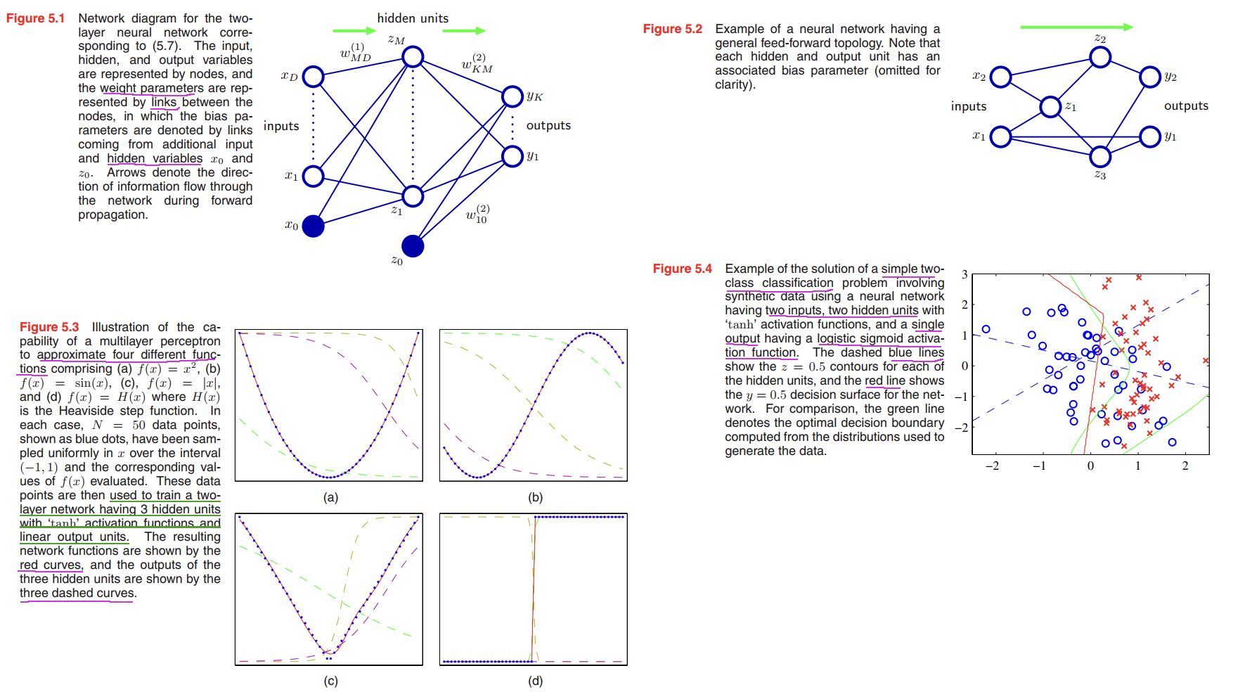
We can give the overall network function that, for sigmoidal output unit activation functions, takes the form
$$
y_k(x,\pmb{w}) = \sigma(\sum_{j=0}^{M} w_{kj}^{(2)}h(\sum_{i=0}^{D}w_{ji}^{(1)}x_i))
\tag{5.9}
$$
A key difference compared to the perceptron, however, is that the neural network uses continuous sigmoidal nonlinearities in the hidden units, whereas the perceptron uses step-function nonlinearities. This means that the neural network function is differentiable with respect to the network parameters, and this property will play a central role in network training.
Network Training
In summary, there is a natural choice of both output unit activation function and matching error function, according to the type of problem being solved.
- For regression. we use linear outputs and a sum-of-squares error.
$$
E(\pmb{w}) = \frac{1}{2}\sum_{n=1}^{N}\lbrace y(x_n, \pmb{w}) - t_n\rbrace^2
\tag{5.14}
$$ - for (multiple independent) binary classifications. we use logistic sigmoid outputs and a cross-entropy error function.
$$
y = \sigma(a) = \frac{1}{1 + exp(-a)}
\tag{5.19}
$$
$$
E(\pmb{w}) = -\sum_{n=1}^{N}\lbrace t_n\ln y_n + (1-t_n)\ln(1-y_n)\rbrace, t_n = 0,1
\tag{5.21}
$$
If we have $K$ separate binary classifications to perform, then we can use a network having $K$ outputs each of which has a logistic sigmoid activation function. Associated with each output is a binary class label $t_k \in {0, 1}$, where $k = 1, . . . , K$.
$$
E(\pmb{w}) = -\sum_{n=1}^{N}\sum_{k=1}^{K} \lbrace t_{nk}\ln y_{nk} + (1 - t_{nk})\ln (1-y_{nk})\rbrace
\tag{5.23}
$$ - for multiclass classification. we use softmax outputs with the corresponding multiclass cross-entropy error function.
$$
y_k(x,\pmb{w}) = \frac{exp(a_k(\pmb{x, w}))}{\sum_j exp(a_j(\pmb{x,w}))}
\tag{5.25}
$$
$$
E(\pmb{w}) = -\sum_{n=1}^{N}\sum_{k=1}^{K} t_{nk} \ln y_k(x_n, \pmb{w})
\tag{5.24}
$$ - For classification problems involving two classes. we can use a single logistic sigmoid output, or alternatively we can use a network with two outputs having a softmax output activation function.
Parameter optimization
if we make a small step in weight space from $\pmb{w}$ to $\pmb{w + \sigma w}$ then the change in the error function is $\sigma E \simeq \sigma \pmb{w^T} \nabla E(\pmb{w})$, where the vector $\nabla E(\pmb{w})$ points in the direction of greatest rate of increase of the error function.
However, the error function typically has a highly nonlinear dependence on the weights and bias parameters, and so there will be many points in weight space at which the gradient vanishes (or is numerically very small).
$$
\nabla E(\pmb{w}) = 0 \tag{5.26}
$$
For a successful application of neural networks, it may not be necessary to find the global minimum (and in general it will not be known whether the global minimum has been found) but it may be necessary to compare several local minima in order to find a sufficiently good solution.
Because there is clearly no hope of finding an analytical solution to the equation $\nabla E(\pmb{w}) = 0$ we resort to iterative numerical procedures.
Most techniques involve choosing some initial value $\pmb{w^{(0)}}$ for the weight vector and then moving through weight space in a succession of steps of the form
$$
\pmb{w}^{(\tau + 1)} = \pmb{w}^{(\tau)} + \Delta \pmb{w^{(\tau)}}
\tag{5.27}
$$
👉More about Gradient in Calculus >>
Local quadratic approximation
Consider the 👉Taylor expansion >> of $E(\pmb{w})$ around some point $\pmb{\hat{w}}$ in weight space
$$
E(\pmb{w}) \simeq E(\pmb{\hat{w}}) + (\pmb{w - \pmb{\hat{w}}})^T \pmb{b} + \frac{1}{2}(\pmb{w - \pmb{\hat{w}}})^T \pmb{H}(\pmb{w - \pmb{\hat{w}}})
\tag{5.28}
$$
where cubic and higher terms have been omitted. Here $\pmb{b}$ is defined to be the gradient of $E$ evaluated at $\pmb{\hat{w}}$
$$
\pmb{b} = \nabla E|_{\pmb{w} = \pmb{\hat{w}}}
\tag{5.29}
$$
and the Hessian matrix $\pmb{H} = \nabla \nabla E$ has elements($\pmb{H}$ is symmetric)
$$
(\pmb{H})_{ij} = \frac{\partial E}{\partial w_i \partial w_j} |_{\pmb{w = \hat{w}}}
\tag{5.30}
$$
From (5.28), the corresponding local approximation to the gradient is given by
$$
\nabla E \simeq \pmb{b} + \pmb{H}(\pmb{w - \hat{w}})
\tag{5.31}
$$
Consider the particular case of a local quadratic approximation around a point $\pmb{w^{\ast}}$ that is a minimum of the error function. In this case there is no linear term, because $\nabla E = 0$ at $\pmb{w^{\ast}}$, and (5.28) becomes
$$
E(\pmb{w}) = E(\pmb{w\ast}) + \frac{1}{2}(\pmb{w-w^{\ast}})^T\pmb{H}(\pmb{w-w^{\ast}})
\tag{5.32}
$$
where the Hessian $\pmb{H}$ is evaluated at $\pmb{w^{\ast}}$.
Consider the eigenvalue equation for Hessian Matrix:
$$
\pmb{Hu_i} = \lambda_i \pmb{u_i}
\tag{5.33}
$$
where the eigenvectors $\pmb{u_i}$ form a complete orthonormal set so that
$$
\pmb{u_i^Tu_j} = \sigma_{ij}
\tag{5.34}
$$
We now expand $(\pmb{w − w^{\ast}})$ as a linear combination of the eigenvectors in the form
$$
\pmb{w-w^{\ast}} = \sum_i \alpha_i \pmb{u_i}
\tag{5.35}
$$
Recall $x = Py$, $x^T A x = y^T D y$, columns of $P$ are the eigen vectors of $A$, $D$ is a diagonal matrix with eigen values.
This can be regarded as a transformation of the coordinate system in which the origin is translated to the point $\pmb{w^{\ast}}$, and the axes are rotated to align with the eigenvectors.
Substituting (5.35) into (5.32), and using (5.33) and (5.34), allows the error function to be written in the form
$$
E(\pmb{w}) = E(\pmb{w^{\ast}}) + \frac{1}{2}\sum_i \lambda_i \alpha_i^2
\tag{5.36}
$$
A matrix $\pmb{H}$ is said to be positive definite if, and only if,
$$
\pmb{v^THv} > 0, for-all-\pmb{v}
\tag{5.37}
$$
Because the eigenvectors $\lbrace \pmb{u_i} \rbrace$ form a complete set, an arbitrary vector $\pmb{v}$ can be written in the form
$$
\pmb{v} = \sum_i c_i \pmb{u_i}
\tag{5.38}
$$
From (5.33) and (5.34), we then have
$$
\pmb{v^THv} = \sum_i c_i^2 \lambda_i
\tag{5.39}
$$
and so $\pmb{H}$ will be positive definite if, and only if, all of its eigenvalues are positive.
For a one-dimensional weight space, a stationary point $\pmb{w^{\ast}}$ will be a minimum if
$$
\frac{\partial^2 E}{\partial \pmb{w^2}}|_{\pmb{w^{\ast}}} > 0
\tag{5.40}
$$
The corresponding result in $D$-dimensions is that the Hessian matrix, evaluated at $\pmb{w^{\ast}}$, should be positive definite.
👉More about Eigenvalues in Algebra >>
👉More about Positive Definite in Algebra >>
Use of gradient information
Gradient descent optimization
The simplest approach to using gradient information is to choose the weight update in (5.27) to comprise a small step in the direction of the negative gradient, so that
$$
\pmb{w}^{\tau + 1} = \pmb{w}^{(\tau)} - \eta \nabla E(\pmb{w}^{(\tau)})
\tag{5.41}
$$
where the parameter $\eta > 0$ is known as the learning rate.
For batch optimization (Techniques that use the whole data set at once are called batch methods), there are more efficient methods, such as conjugate gradients and quasi-Newton methods, which are much more robust and much faster than simple gradient descent.
Unlike gradient descent, these algorithms have the property that the error function always decreases at each iteration unless the weight vector has arrived at a local or global minimum.
There is, however, an on-line version of gradient descent that has proved useful in practice for training neural networks on large data sets. On-line gradient descent, also known as sequential gradient descent or stochastic gradient descent, makes an update to the weight vector based on one data point at a time, so that
$$
\pmb{w}^{\tau + 1} = \pmb{w}^{\tau} - \eta \nabla E_n(\pmb{w}^{(\tau)})
\tag{5.43}
$$
- One advantage of on-line methods compared to batch methods is that the former handle redundancy in the data much more efficiently.
- Another property of on-line gradient descent is the possibility of escaping from local minima, since a stationary point with respect to the error function for the whole data set will generally not be a stationary point for each data point individually.
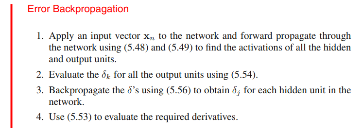
Error Backpropagation
Evaluation of error-function derivatives
Consider first a simple linear model in which the outputs $y_k$ are linear combinations of the input variables $x_i$ so that
$$
y_k = \sum_i w_{ki}x_i
\tag{5.45}
$$
together with an error function that, for a particular input pattern $n$, takes the form
$$
E_n = \frac{1}{2}\sum_k (y_{nk} - t_{nk})^2, y_{nk} = y_k(x_n, \pmb{w})
\tag{5.46}
$$
The gradient of this error function with respect to a weight $w_{ji}$ is given by
$$
\frac{\partial E_n}{\partial w_{ji}} = (y_{nj}-t_{nj})x_{ni}
\tag{5.47}
$$
which can be interpreted as a ‘local’ computation involving the product of an ‘error signal’ $y_{nj} − t_{nj}$ associated with the output end of the link $w_{ji}$ and the variable $x_{ni}$ associated with the input end of the link.
In a general feed-forward network, each unit computes a weighted sum of its inputs of the form
$$
a_j = \sum_i w_{ji}z_i
\tag{5.48}
$$
where $z_i$ is the activation of a unit, or input, that sends a connection to unit $j$, and $w_{ji}$ is the weight associated with that connection.
The sum in (5.48) is transformed by a nonlinear activation function $h(\cdot)$ to give the activation $z_j$ of unit $j$ in the form
$$
z_j = h(a_j)
\tag{5.49}
$$
We can therefore apply the 👉chain rule >> for partial derivatives to give
$$
\frac{\partial E_n}{\partial w_{ji}} = \frac{\partial E_n}{\partial a_j} \frac{\partial a_j}{\partial w_{ji}}
\tag{5.50}
$$
let $\delta_j$ be errors,
$$
\delta_j \equiv \frac{\partial E_n}{\partial a_j}
\tag{5.51}
$$
By equation(5.48), we get
$$
\frac{\partial a_j}{\partial w_{ji}} = z_i
\tag{5.52}
$$
Substituting (5.51) and (5.52) into(5.50), we obtain
$$
\frac{\partial E_n}{\partial w_{ji}} = \delta_j z_i
\tag{5.53}
$$
Equation (5.53) has the same form with equation(5.47), right?
As we have seen already, for the output units, we have
$$
\delta_k = y_k - t_k
\tag{5.54}
$$
To evaluate the $\sigma$’s for hidden units, we again make use of the chain rule for partial derivatives,
$$
\delta_j \equiv \frac{\partial E_n}{\partial a_j} = \sum_k \frac{\partial E_n}{\partial a_k} \frac{\partial a_k}{\partial a_j}
\tag{5.55}
$$
where the sum runs over all units $k$ to which unit $j$ sends connections.
If we now substitute the definition of $\sigma$ given by (5.51) into (5.55), and make use of (5.48) and (5.49), we obtain the following backpropagation formula
$$
\delta_j = h’(a_j)\sum_k w_{kj} \delta_k
\tag{5.56}
$$
which tells us that the value of $\sigma$ for a particular hidden unit can be obtained by propagating the $\sigma$’s backwards from units higher up in the network, as illustrated in Figure 5.7.
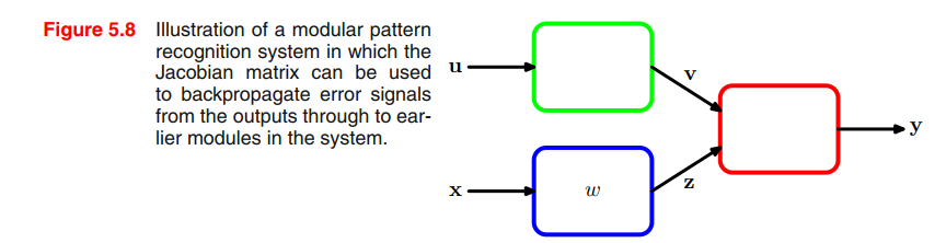
A simple example
Consider a two-layer network of the form illustrated in Figure 5.1, together with a sum-of-squares error, in which the output units have linear activation functions, so that $y_k = a_k$, while the hidden units have logistic sigmoid activation functions given by
$$
h(a) \equiv tanh(a)
\tag{5.58}
$$
where
$$
tanh(a) = \frac{e^a - e^{-a}}{e^a + e^{-a}}
\tag{5.59}
$$
this activation function’s derivative is,
$$
h(a) = 1 - h(a)^2
\tag{5.60}
$$
for pattern n the sum-of-squares error function is given by
$$
E_n = \frac{1}{2} \sum_{k=1}^K (y_k - t_k)^2
\tag{5.61}
$$
where $y_k$ is the activation of output unit $k$, and $t_k$ is the corresponding target, for a particular input pattern $x_n$.
For each pattern in the training set in turn, we first perform a forward propagation using
$$
a_j = \sum_{i = 0}^D w_{ji}^{(1)} x_i
\tag{5.62}
$$
$$
z_j = tanh(a_j)
\tag{5.63}
$$
$$
y_k = \sum_{j=1}^M w_{kj}^{(2)} z_j
\tag{5.64}
$$
Next we compute the $\sigma$’s for each output unit using
$$
\sigma_k = y_k - t_k
\tag{5.65}
$$
Then we backpropagate these to obtain $\sigma s$ for the hidden units using
$$
\sigma_j = (1 - z_j^2) \sum_{k=1}^K w_{kj} \sigma_k
\tag{5.66}
$$
Finally, the derivatives with respect to the first-layer and second-layer weights are given by
$$
\frac{\partial E_n}{\partial w_{ji}^{(1)}} = \sigma_j x_i
$$
$$
\frac{\partial E_n}{\partial w_{kj}^{(2)}} = \sigma_k z_j
\tag{5.67}
$$
Efficiency of backpropagation
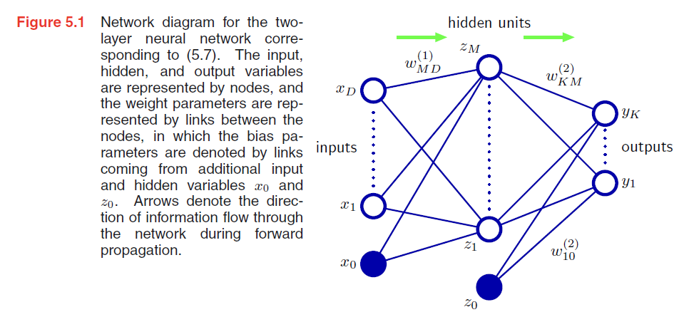
The Jacobian matrix
The technique of backpropagation can also be applied to the calculation of other derivatives.
Here we consider the evaluation of the Jacobian matrix, whose elements are given by the derivatives of the network outputs with respect to the inputs
$$
J_{ki} \equiv \frac{\partial y_k}{\partial x_i}
\tag{5.70}
$$
Jacobian matrices play a useful role in systems built from a number of distinct modules, as illustrated in Figure 5.8.
Suppose we wish to minimize an error function $E$ with respect to the parameter $w$ in Figure 5.8. The derivative of the error function is given by
$$
\frac{\partial E}{\partial w} = \sum_{k,j} \frac{\partial E}{\partial y_k}\frac{\partial y_k}{\partial z_j}\frac{\partial z_j}{\partial w}
\tag{5.71}
$$
In general, the network mapping represented by a trained neural network will be nonlinear, and so the elements of the Jacobian matrix will not be constants but will depend on the particular input vector used.
$$
\begin{aligned}
J_{ki} &= \frac{\partial y_k}{\partial x_i}\\
&= \sum_j \frac{\partial y_k}{\partial a_j}\frac{\partial a_j}{\partial x_i}\\
&= \sum_j w_{ji}\frac{\partial y_k}{\partial a_j}
\end{aligned}
\tag{5.73}
$$
We now write down a recursive backpropagation formula to determine the derivatives $\frac{\partial y_k}{\partial a_j}$
$$
\begin{aligned}
\frac{\partial y_k}{\partial a_j} &= \sum_l \frac{\partial y_k}{\partial a_l} \frac{\partial a_l}{\partial a_j}\\
&= h’(a_j)\sum_l w_{lj}\frac{\partial y_k}{\partial a_l}
\end{aligned}
\tag{5.74}
$$
👉Jacobian matrix in Numberical Analysis >>
The Hessian Matrix
The Hessian plays an important role in many aspects of neural computing, including the following:
- Several nonlinear optimization algorithms used for training neural networks are based on considerations of the second-order properties of the error surface, which are controlled by the Hessian matrix (Bishop and Nabney, 2008).
- The Hessian forms the basis of a fast procedure for re-training a feed-forward network following a small change in the training data (Bishop, 1991).
- The inverse of the Hessian has been used to identify the least significant weights in a network as part of network ‘pruning’ algorithms (Le Cun et al., 1990).
- The Hessian plays a central role in the Laplace approximation for a Bayesian neural network (see Section 5.7). Its inverse is used to determine the predictive distribution for a trained network, its eigenvalues determine the values of hyperparameters, and its determinant is used to evaluate the model evidence.
Diagonal approximation
From (5.48), the diagonal elements of the Hessian, for pattern $n$, can be written
$$
\frac{\partial^2 E_n}{\partial w^2_{ji}} = \frac{\partial^2 E_n}{\partial a^2_j} z^2_i
\tag{5.79}
$$
recursively using the chain rule of differential calculus to give a backpropagation equation of the form
$$
\frac{\partial^2 E_n}{\partial a^2_j} = h’(a_j)^2 \sum_k \sum_{k’} w_{kj}w_{k’j} \frac{\partial^2 E_n}{\partial a_k \partial a_{k’}} + h’’(a_j) \sum_k w_{kj} \frac{\partial^2 E_n}{\partial a_k}
\tag{5.80}
$$
If we now neglect off-diagonal elements in the second-derivative terms,
$$
\frac{\partial^2 E_n}{\partial a^2_j} = h’(a_j)^2 \sum_k w^2_{kj} \frac{\partial^2 E_n}{\partial^2 a_k} + h’’(a_j) \sum_k w_{kj} \frac{\partial E_n}{\partial a_k}
\tag{5.81}
$$
The major roblem with diagonal approximations, however, is that in practice the Hessian is typically found to be strongly nondiagonal, and so these approximations, which are driven mainly be computational convenience, must be treated with care.
Outer product approximation
When neural networks are applied to regression problems, it is common to use a sum-of-squares error function of the form
$$
E = \frac{1}{2} \sum_{n=1}^N(y_n - t_n)^2
\tag{5.82}
$$
We can then write the Hessian matrix in the form
$$
\pmb{H} = \nabla \nabla E = \sum_{n=1}^{N} \nabla y_n \nabla y_n + \sum_{n=1}^N (y_n - t_n)\nabla \nabla y_n
\tag{5.83}
$$
By neglecting the second term in (5.83), we arrive at the Levenberg–Marquardt approximation or outer product approximation (because the Hessian matrix is built up from a sum of outer products of vectors), given by
$$
\pmb{H} \simeq \sum_{n=1}^N \pmb{b_n b_n^T}, \pmb{b_n} = \nabla y_n = \nabla a_n
\tag{5.84}
$$
Evaluation of the outer product approximation for the Hessian is straightforward as it only involves first derivatives of the error function,which can be evaluated efficiently in $O(W)$ steps using standard backpropagation.
It is important to emphasize that this approximation is only likely to be valid for a network that has been trained appropriately.
Inverse Hessian
First we write the outer-product approximation in matrix notation as
$$
\pmb{H_N} = \sum_{n=1}^N \pmb{b_n b_n^T}
\tag{5.86}
$$
where $\pmb{b_n} \equiv ∇_{\pmb{w}}a_n$ is the contribution to the gradient of the output unit activation arising from data point $n$.
Suppose we have already obtained the inverse Hessian using the first $L$ data points. By separating off the contribution from data point $L + 1$, we obtain
$$
\pmb{H} _{L+1} = \pmb{H} _L + \pmb{b} _{L+1} \pmb{b^T} _{L+1}
\tag{5.87}
$$
In order to evaluate the inverse of the Hessian, we now consider the matrix identity
$$
(\pmb{M+vv^T})^{-1} = \pmb{M}^{-1}- \frac{(\pmb{M^{-1}v})(\pmb{v^TM^{-1}})}{1+\pmb{v^TM^{-1}v}}
\tag{5.88}
$$
If we now identify $\pmb{H_{L}}$ with $\pmb{M}$ and $\pmb{b}_{L+1}$ with $\pmb{v}$, we obtain
$$
\pmb{H_{L+1}}^{-1} = \pmb{H_L}^{-1}- \frac{(\pmb{H_L^{-1}b_{L+1}})(\pmb{b_{L+1}^TH_L^{-1}})}{1+\pmb{b_{L+1}^TH_L^{-1}b_{L+1}}}
\tag{5.89}
$$
In this way, data points are sequentially absorbed until $L+1 = N$ and the whole data set has been processed.
In particular, quasi-Newton nonlinear optimization algorithms gradually build up an approximation to the inverse of the Hessian during training.
Finite differences
Exact evaluation of the Hessian
Fast multiplication by the Hessian
For many applications of the Hessian, the quantity of interest is not the Hessian matrix $\pmb{H}$ itself but the product of $\pmb{H}$ with some vector $\pmb{v}$.
Regularization in Neural Networks
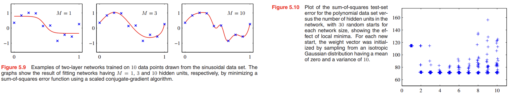
Note that $M$ controls the number of parameters (weights and biases) in the network, and so we might expect that in a maximum likelihood setting there will be an optimum value of $M$ that gives the best generalization performance, corresponding to the optimum balance between under-fitting and over-fitting.
Consistent Gaussian priors
Remember in Chapter1, we see that an alternative approach is to choose a relatively large value for $M$ and then to control complexity by the addition of a regularization term to the error function. The simplest regularizer is the quadratic, giving a regularized error of the form
$$
\widetilde{E}(\pmb{w}) = E(\pmb{w}) + \frac{\lambda}{2}\pmb{w^Tw}
\tag{5.112}
$$
This regularizer is also known as weight decay. One limitation of this form is inconsistent with certain scaling properties of network mappings.
Consider a multilayer perceptron network having two layers of weights and linear output units. The activations of the hidden units in the first hidden layer take the form
$$
z_j = h(\sum_i w_{ji}x_i + w_{j0})
\tag{5.113}
$$
while the activations of the output units are given by
$$
y_k = \sum_j w_{kj}z_j + w_{k0}
\tag{5.114}
$$
Suppose we perform a linear transformation of the input data of the form
$$
x_i \rightarrow \widetilde{x_i} = ax_i + b
\tag{5.115}
$$
$$
y_k \rightarrow \widetilde{y_k} = cy_k + d
\tag{5.118}
$$
also, we can perform a corresponding linear transformation of output data and the weights parameters.
If we train one network using the original data and one network using data for which the input and/or target variables are transformed by one of the above linear transformations, then consistency requires that we should obtain equivalent networks that differ only by the linear transformation of the weights as given.
Any regularizer should be consistent with this property.
These require that the regularizer should be invariant to re-scaling of the weights and to shifts of the biases. Such a regularizer is given by
$$
\frac{\lambda_1}{2} \sum_{w \in \mathcal{W_1}} w^2 + \frac{\lambda_2}{2} \sum_{w \in \mathcal{W_2}} w^2
\tag{5.121}
$$
where $\mathcal{W_1}$ denotes the set of weights in the first layer, $\mathcal{W_2}$ denotes the set of weights in the second layer, and biases are excluded from the summations.
This regularizer will remain unchanged under the weight transformations provided the regularization parameters are re-scaled using
$$
\lambda_1 \rightarrow a^{1/2}\lambda_1\\
\lambda_2 \rightarrow c^{-1/2}\lambda_2
$$
The regularizer (5.121) corresponds to a prior of the form
$$
p(\pmb{w}|\alpha_1, \alpha_2) \propto exp(-\frac{\alpha_1}{2}\sum_{w \in \mathcal{W_1}} w^2 - \frac{\alpha_2}{2}\sum_{w \in \mathcal{W_2}} w^2)
\tag{5.122}
$$
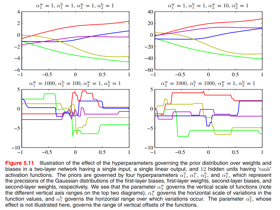
We can illustrate the effect of the resulting four hyperparameters by drawing samples from the prior and plotting the corresponding network functions, as shown in Figure 5.11.
More generally, we can consider priors in which the weights are divided into any number of groups $\mathcal{W_k}$ so that
$$
p(\pmb{w}) \propto exp(-\frac{1}{2}\sum_k \alpha_k ||\pmb{w}||_k^2)
\tag{5.123}
$$
where,
$$
||\pmb{w}|| _k^2 = \sum_{j \in \mathcal{W_k}} w_j^2
\tag{5.124}
$$
Early stopping
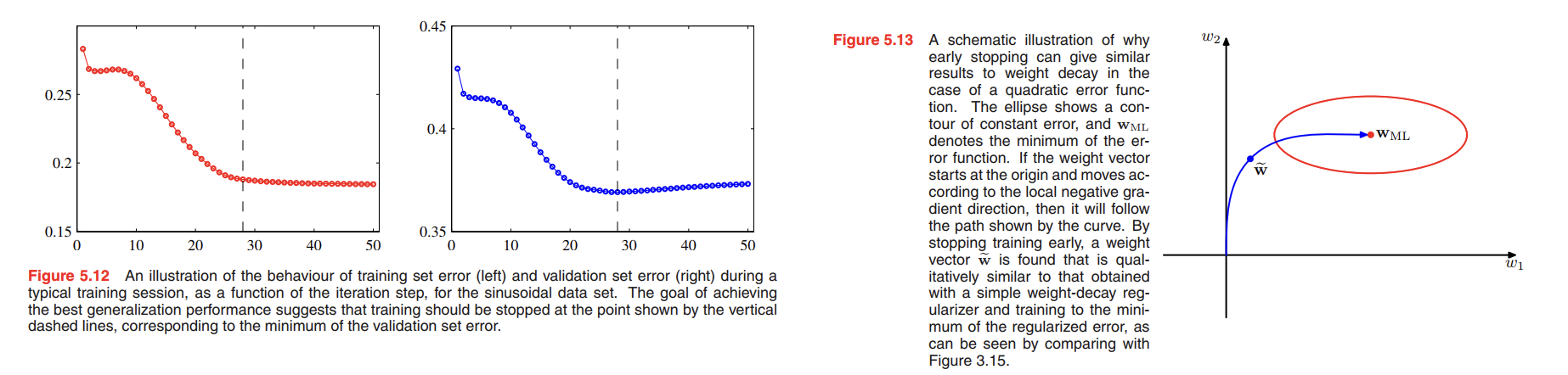
An alternative to regularization as a way of controlling the effective complexity of a network is the procedure of early stopping.
Invariances
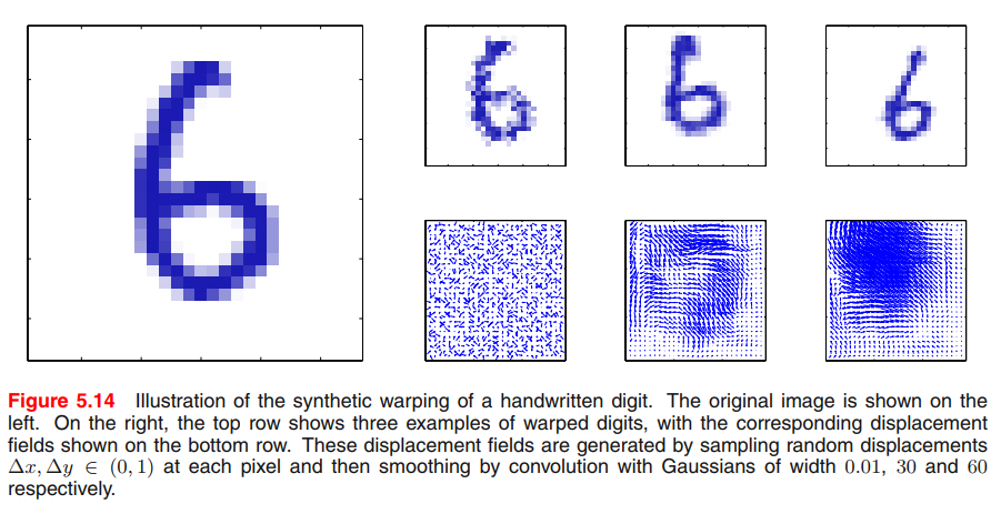
For example, in the classification of objects in two-dimensional images, such as handwritten digits, a particular object should be assigned the same classification irrespective of its position within the image (translation invariance) or of its size (scale invariance).
Such transformations produce significant changes in the raw data, expressed in terms of the intensities at each of the pixels in the image, and yet should give rise to the same output from the classification system.
We therefore seek alternative approaches for encouraging an adaptive model to exhibit the required invariances. These can broadly be divided into four categories:
- The training set is augmented using replicas of the training patterns, transformed according to the desired invariances. For instance, in our digit recognition example, we could make multiple copies of each example in which the digit is shifted to a different position in each image.
- A regularization term is added to the error function that penalizes changes in the model output when the input is transformed. This leads to the technique of tangent propagation, discussed in Section 5.5.4.
- Invariance is built into the pre-processing by extracting features that are invariant under the required transformations. Any subsequent regression or classification system that uses such features as inputs will necessarily also respect these invariances.
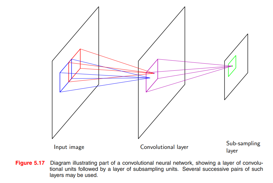
- The final option is to build the invariance properties into the structure of a neural network (or into the definition of a kernel function in the case of techniques such as the relevance vector machine). One way to achieve this is through the use of local receptive fields and shared weights, as discussed in the context of convolutional neural networks in Section 5.5.6.
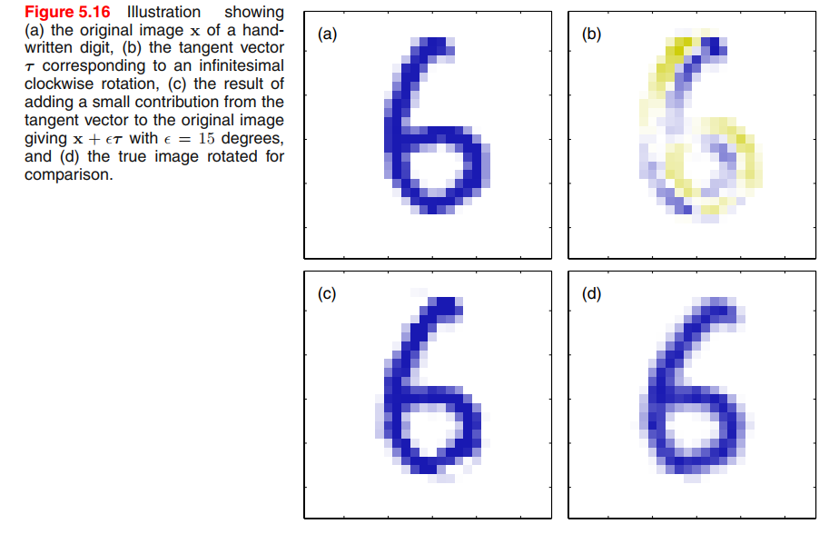
Tangent propagation
Suppose the transformation is governed by a single parameter $\xi$ (which might be rotation angle for instance). Then the subspace $\mathcal{M}$ swept out by $x_n$ will be one-dimensional, and will be parameterized by $\xi$.
Let the vector that results from acting on $x_n$ by this transformation be denoted by $s(x_n, \xi)$, which is defined so that $s(x_n, 0) = x$. Then the tangent to the curve $M$ is given by the 👉directional derivative >> $\tau = \frac{\partial s}{\partial \xi}$, and the tangent vector at the point $x_n$ is given by
$$
\tau_n = \frac{\partial s(x_n, \xi)}{\partial \xi}|_{\xi = 0}
\tag{5.125}
$$
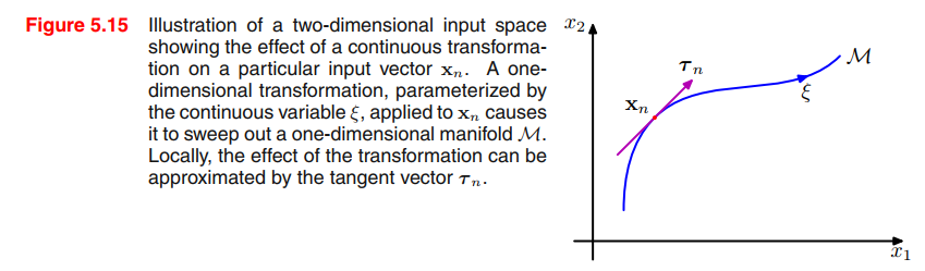
Image a function $z = f(x,y)$, the directional derivative is $D_{\pmb{u}}f|P_0$, is the slope of the trace curve on the surface at point $P_0$.
The derivative of output $k$ with respect to $\xi$ is given by
$$
\frac{\partial y_k}{\partial \xi} |_{\xi = 0} = \sum_{i=1}^D \frac{\partial y_k}{\partial x_i}\frac{\partial x_i}{\partial \xi}|_{\xi = 0} = \sum_{i=1}^D J_{ki}\tau_i
\tag{5.126}
$$
where $J_{ki}$ is the $(k, i)$ element of the Jacobian matrix $J$.
The result (5.126) can be used to modify the standard error function, so as to encourage local invariance in the neighbourhood of the data points, by the addition to the original error function $E$ of a regularization function $\Omega$ to give a total error function of the form
$$
\widetilde{E} = E + \lambda \Omega
\tag{5.127}
$$
where $\lambda$ is a regularization coefficient and
$$
\begin{aligned}
\Omega &= \frac{1}{2} \sum_n \sum_k (\frac{\partial y_{nk}}{\partial \xi}|_{\xi = 0})^2 \\
&= \frac{1}{2} \sum_n \sum_k (\sum_{i=1}^D J_{nki}\tau _{ni})^2
\end{aligned}
\tag{5.128}
$$
The regularization function will be zero when the network mapping function is invariant under the transformation in the neighbourhood of each pattern vector, and the value of the parameter $\lambda$ determines the balance between fitting the training data and learning the invariance property.
A related technique, called tangent distance, can be used to build invariance properties into distance-based methods such as nearest-neighbour classifiers (Simardet al., 1993).
Training with transformed data
Encourage invariance of a model to a set of transformations is to expand the training set using transformed versions of the original
input patterns, this approach is closely related to the technique of tangent propagation.
Convolutional networks
Another approach to creating models that are invariant to certain transformation of the inputs is to build the invariance properties into the structure of a neural network. This is the basis for the convolutional neural network (Le Cun et al., 1989; LeCun et al., 1998), which has been widely applied to image data.
Soft weight sharing
Recall that the simple weight decay regularizer, given in (5.112), can be viewed as the negative log of a Gaussian prior distribution over the weights.
We can encourage the weight values to form several groups, rather than just one group, by considering instead a probability distribution that is a mixture of Gaussians.
The centres and variances of the Gaussian components, as well as the mixing coefficients, will be considered as adjustable parameters to be determined as part of the learning process. Thus, we have a probability density of the form
$$
p(\pmb{w}) = \prod_i p(w_i)
\tag{5.136}
$$
where
$$
p(w_i) = \sum_{j=1}^M \pi_j N(w_i | \mu_j, \sigma_j^2)
\tag{5.137}
$$
Taking the negative logarithm then leads to a regularization function of the form
$$
\Omega (\pmb{w}) = - \sum_i \ln (\sum_{j=1}^M \pi_j N(w_j|\mu_j, \sigma_j^2))
\tag{5.138}
$$
The total error function is then given by
$$
\widetilde{E}(\pmb{w}) = E(\pmb{w}) + \lambda \Omega (\pmb{w})
\tag{5.139}
$$
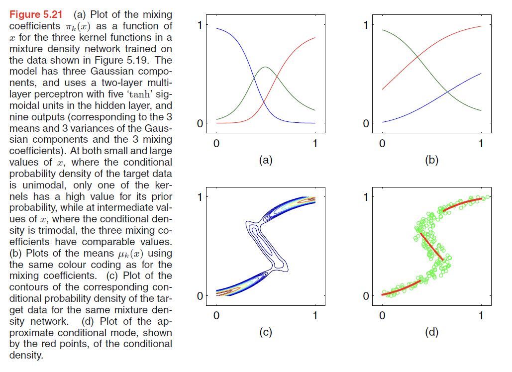
Mixture Density Networks
The goal of supervised learning is to model a conditional distribution $p(T|X)$, which for many simple regression problems is chosen to be Gaussian.(maximum likelihood function, posterior distribution, predictive distribution…)
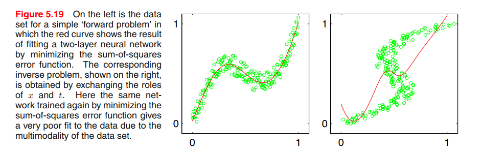
However, practical machine learning problems can often have significantly non-Gaussian distributions. These can arise, for example, with inverse problems in which the distribution can be multimodal(多模态), in which case the Gaussian assumption can lead to very poor predictions.
For example, Data for this problem is generated by sampling a variable $x$ uniformly over the interval $(0, 1)$, to give a set of values ${x_n}$, and the corresponding target values tn are obtained by computing the function $x_n + 0.3 \sin(2\pi x_n)$ and then adding uniform noise over the interval $(−0.1, 0.1)$.
The inverse problem is then obtained by keeping the same data points but exchanging the roles of $x$ and $t$.
Least squares corresponds to maximum likelihood under a Gaussian assumption. We see that this leads to a very poor model for the highly non-Gaussian inverse problem.
We therefore seek a general framework for modelling conditional probability distributions. This can be achieved by using a mixture model for $p(\pmb{t|x})$ in which both the mixing coefficients as well as the component densities are flexible functions of the input vector $\pmb{x}$, giving rise to the mixture density network.
For any given value of $\pmb{x}$, the mixture model provides a general formalism for modelling an arbitrary conditional density function $p(\pmb{t|x})$. Provided we consider a sufficiently flexible network, we then have a framework for approximating arbitrary conditional distributions. Here we shall develop the model explicitly for Gaussian components, so that
$$
p(\pmb{t|x}) = \sum_{k=1}^K \pi_k(\pmb{x}) N(\pmb{t}|\pmb{\mu_k}, \sigma_k^2(\pmb{x}))
\tag{5.148}
$$
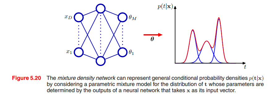
The neural network in Figure 5.20 can, for example, be a two-layer network having sigmoidal (‘tanh’) hidden units. If there are $L$(e.g. L = 1, only Gaussian) components in the mixture model (5.148), and if $t$ has $K$(e.g. K = 3, 3 gaussian distribution mixture) components. Then the network will have $L$ output unit activations denoted by $a_k^{\pi}$ that determine the mixing coefficients $\pi_k(x)$, K outputs denoted by $a_k^{\sigma}$ that determine the kernel widths $\sigma_k(x)$, and $L \times K$ outputs denoted by $a_{kj}^{\mu}$ that determine the components $\mu_{kj}(x)$ of the kernel centres $\mu_k(x)$. ???
The mixing coefficients must satisfy the constraints
$$
\sum_{k=1}^K \pi_k(x) = 1
\tag{5.149}
$$
which can be achieved using a set of softmax outputs
$$
\pi_k(x) = \frac{exp (a_k^\pi)}{\sum_{l=1}^K exp(a_l^\pi)}
\tag{5.150}
$$
Similarly, the variances must satisfy $\sigma_k^2(x) \geq 0$ and so can be represented in terms of the exponentials of the corresponding network activations using
$$
\sigma_k(x) = exp(a_k^{\sigma})
\tag{5.151}
$$
Finally, because the means $\mu_k(x)$ have real components, they can be represented directly by the network output activations
$$
\mu_{kj}(x) = a_{kj}^{\mu}
$$
Bayesian Neural Networks
Posterior parameter distribution
Consider the problem of predicting a single continuous target variable $t$ from a vector $\pmb{x}$ of inputs (the extension to multiple targets is straightforward). We shall suppose that the conditional distribution $p(t|\pmb{x})$ is Gaussian, with an $x$-dependent mean given by the output of a neural network model $y(\pmb{x},\pmb{w})$, and with precision (inverse variance) $\beta$.
We can find a Gaussian approximation to the posterior distribution by using the 👉Laplace approximation >> .
$$
p(\pmb{w} | D, \alpha, \beta) \propto p(\pmb{w} | \alpha) p(D | \pmb{w}, \beta)
\tag{5.164}
$$
$$
q(\pmb{w} | D) = N( \pmb{w} | \pmb{w_{MAP}}, \pmb{A}^{-1})
\tag{5.167}
$$
However, even with the Gaussian approximation to the posterior, this integration is still analytically intractable due to the nonlinearity of the network function $y(\pmb{x}, \pmb{w})$ as a function of $\pmb{w}$.
$$
p(t|\pmb{x}, D) = \int p(t|\pmb{x, w}) q(\pmb{w}|D) d\pmb{w}
\tag{5.168}
$$
To make progress, we now assume that the posterior distribution has small variance compared with the characteristic scales of $\pmb{w}$ over which $y(\pmb{x}, \pmb{w})$ is varying. This allows us to make a Taylor series expansion of the network function around $\pmb{w_{MAP}}$ and retain only the linear terms
$$
y(\pmb{x}, \pmb{w}) \simeq y(\pmb{x}, \pmb{w_{MAP}}) + \pmb{g^T(w - w_{MAP})}
\tag{5.169}
$$
where we have defined
$$
\pmb{g} = \nabla _w y(\pmb{x, w})|_wMAP
\tag{5.170}
$$
With this approximation, we now have a linear-Gaussian model with a Gaussian distribution for $p(\pmb{w})$ and a Gaussian for $p(t|\pmb{w})$ whose mean is a linear function of $\pmb{w}$ of the form
$$
p(t | \pmb{x},\pmb{w}, \beta) \simeq N(t | y(\pmb{x, w_{MAP}} + \pmb{g^T(w-w_{MAP})}), \beta^{-1})
\tag{5.171}
$$
We can therefore make use of the general result (2.115) for the marginal $p(t)$ to give
👉2.115 >>
$$
p(t | \pmb{x}, D, \alpha, \beta) = N(t | y(\pmb{x} , \pmb{w_{MAP}}), \sigma^2(\pmb{x}))
\tag{5.172}
$$
where
$$
\sigma^2{\pmb{x}} = \beta^{-1} + \pmb{g^TA^{-1}g}
\tag{5.173}
$$
Hyperparameter optimization
So far, we have assumed that the hyperparameters $\alpha$ and $\beta$ are fixed and known. We can make use of the evidence framework, discussed in Section 3.5, together with the Gaussian approximation to the posterior obtained using the Laplace approximation, to obtain a practical procedure for choosing the values of such hyperparameters.

