Keywords: Gaussian processes, Radial Basis Function Networks, Laplace approximation, Python
This is the Chapter6 ReadingNotes from book Bishop-Pattern-Recognition-and-Machine-Learning-2006. [Code_Python]
Dual Representations(二元表示)
Many linear parametric models can be re-cast into an equivalent ‘dual representation’ in which the predictions are also based on linear combinations of a kernel function evaluated at the training data points.
There are numerous forms of kernel functions in common use, and we shall encounter several examples in this chapter. Many have the property of being a function only of the difference between the arguments, so that $k(\pmb{x}, \pmb{x’}) = k(\pmb{x − x’})$, which are known as stationary kernels because they are invariant to translations in input space.
A further specialization involves homogeneous kernels, also known as radial basis functions, which depend only on the magnitude of the distance (typically Euclidean) between the arguments so that $k(\pmb{x}, \pmb{x’}) = k(||\pmb{x − x’}||)$.
Here we consider a linear regression model whose parameters are determined by minimizing a regularized sum-of-squares error function given by
$$
J(\pmb{w}) = \frac{1}{2}\sum_{n=1}^N \lbrace \pmb{w}^T\phi(x_n) - t_n\rbrace^2 + \frac{\lambda}{2} \pmb{w^Tw}
\tag{6.2}
$$
If we set the gradient of $J(\pmb{w})$ with respect to $\pmb{w}$ equal to zero,
$$
\begin{aligned}
\pmb{w} &= -\frac{1}{\lambda} \sum_{n=1}^{N} \lbrace \pmb{w^T}\phi(x_n) - t_n\rbrace \phi(x_n)\\
&= \sum_{n=1}^N a_n\phi(x_n) \\
&= \pmb{\Phi^Ta}
\end{aligned}
\tag{6.3}
$$
where $\pmb{\Phi}$ is the design matrix, whose $n^{th}$ row is given by $\phi(x_n)^T$. Here the vector $\pmb{a} = (a_1, \cdots, a_N)^T$, and we have defined
$$
a_n = -\frac{1}{\lambda} \lbrace \pmb{w^T\phi(x_n) - t_n}\rbrace
\tag{6.4}
$$
If we substitute $\pmb{w = \Phi^Ta}$ into $J(\pmb{w})$, we obtain
$$
J(\pmb{a}) = \frac{1}{2}\pmb{a^T\Phi \Phi^T \Phi \Phi^T a - a^T\Phi \Phi^T T + \frac{1}{2} T^TT + \frac{\lambda}{2}a^T \Phi \Phi^Ta}
\tag{6.5}
$$
We now define the Gram matrix $\pmb{K = \Phi \Phi^T}$, which is an $N × N$ symmetric matrix with elements
$$
K_{nm} = \phi(x_n)^T \phi(x_m) = k(x_n, x_m)
\tag{6.6}
$$
the kernel function is
$$
k(x,x’) = \phi(x)^T \phi(x’)
\tag{6.1}
$$
In terms of the Gram matrix, the sum-of-squares error function can be written as
$$
J(\pmb{a}) = \frac{1}{2}\pmb{a^T KK a - a^T K T + \frac{1}{2} T^TT + \frac{\lambda}{2}a^T K a}
\tag{6.7}
$$
Setting the gradient of $J(\pmb{a})$ with respect to a to zero, we obtain the following solution
$$
\pmb{a} = (\pmb{K} + \lambda \pmb{I_N})^{-1}T
\tag{6.8}
$$
If we substitute this back into the linear regression model, we obtain the following prediction for a new input $x$
$$
\begin{aligned}
y(x) &= \pmb{w^T}\phi(x) \\
&= \pmb{a^T}\Phi \phi(x) \\
&= k(x)^T (\pmb{K} + \lambda \pmb{I_N})^{-1}T
\end{aligned}
\tag{6.9}
$$
Thus we see that the dual formulation allows the solution to the least-squares problem to be expressed entirely in terms of the kernel function $k(x, x’)$.
We can therefore work directly in terms of kernels and avoid the explicit introduction of the feature vector $\phi(x)$, which allows us implicitly to use feature spaces of high, even infinite, dimensionality.
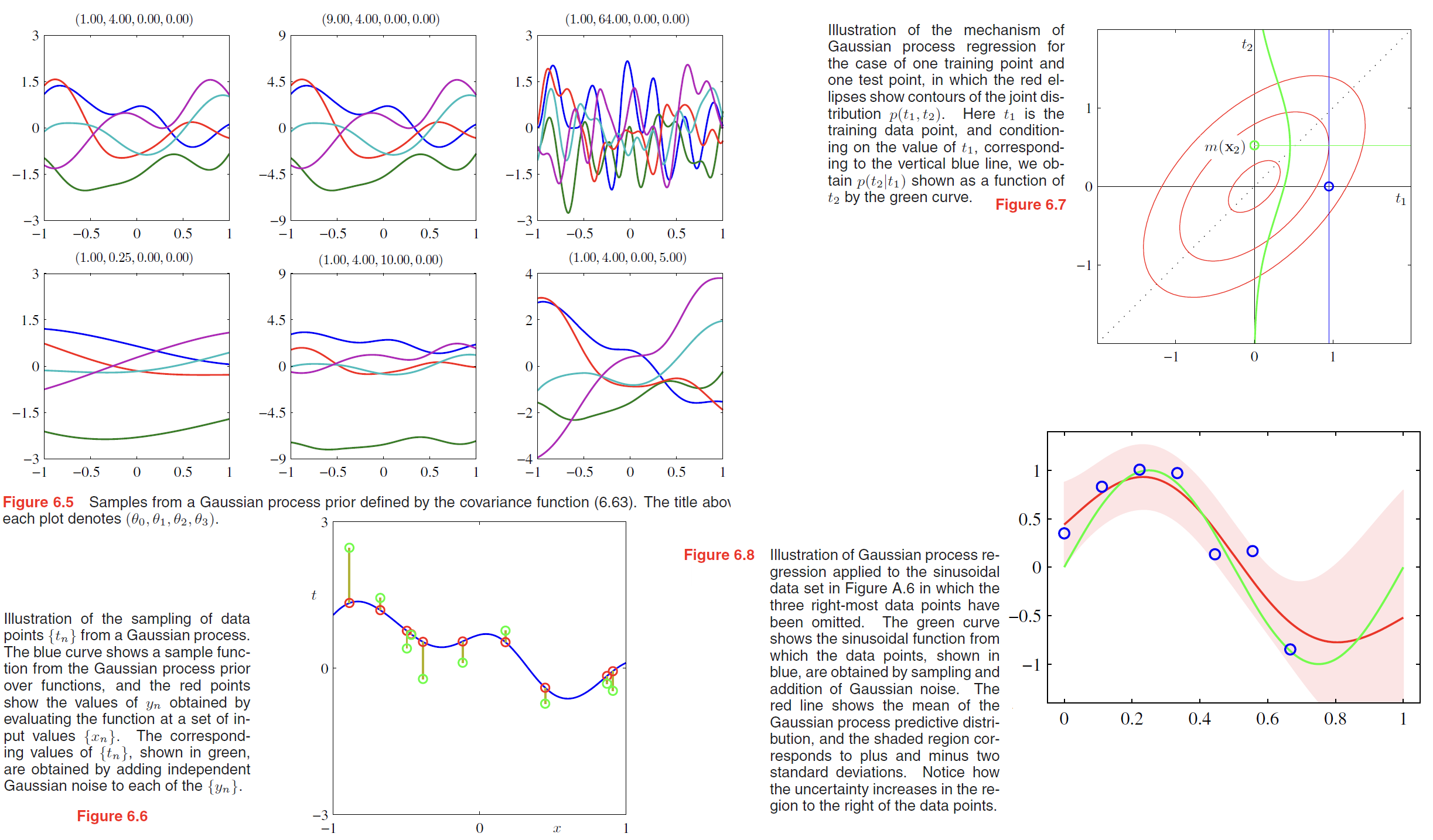
Constructing Kernels
One approach is to choose a feature space mapping $\phi(x)$ and then use this to find the corresponding kernel, as is illustrated in Figure 6.1. Here the kernel function is defined for a one-dimensional input space by
$$
k(x,x’) = \phi(x)^T \phi(x’) = \sum_{i=1}^M \phi_i(x) \phi_i(x’)
\tag{6.10}
$$
where $\phi_i(x)$ are the basis functions.
For example, consider a kernel function given by
$$
k(\pmb{x,z}) = (\pmb{x^Tz})^2
\tag{6.11}
$$
If we take the particular case of a two-dimensional input space $\pmb{x} = (x_1, x_2)$ we can expand out the terms and thereby identify the corresponding nonlinear feature mapping
$$
\begin{aligned}
k(\pmb{x,z}) &= (\pmb{x^Tz})^2\\
&=(x_1 z_1 + x_2 z_2)^2\\
&= (x_1^2, \sqrt{2}x_1x_2, x_2^2)(z_1^2, \sqrt{2}z_1z_2, z_2^2)^T\\
&= \phi(\pmb{x})^T\phi(\pmb{z})
\end{aligned}
\tag{6.12}
$$
Equipped with these properties, we can now embark on the construction of more complex kernels appropriate to specific applications.
We saw that the simple polynomial kernel $k(\pmb{x, x’}) = (\pmb{x^Tx’})^2$ contains only terms of degree two.
Similarly, $k(\pmb{x, x’}) = (\pmb{x^Tx’})^M$ contains all monomials of order $M$.
For instance, if $\pmb{x}$ and $\pmb{x’}$ are two images, then the kernel represents a particular weighted sum of all possible products of $M$ pixels in the first image with $M$ pixels in the second image.
Another commonly used kernel takes the form is often called a ‘Gaussian’ kernel,
$$
k(\pmb{x, x’}) = exp(-||\pmb{x-x’}||^2 / 2\sigma^2)
\tag{6.23}
$$
Since,
$$
||\pmb{x - x’}||^2 = \pmb{x^Tx} + (\pmb{x’^Tx’}) - 2\pmb{x^Tx’}
\tag{6.24}
$$
then,
$$
k(\pmb{x, x’}) = exp(-\pmb{x^Tx}/2\sigma^2)exp(\pmb{x^Tx’}/\sigma^2)exp(-\pmb{x’^Tx’}/2\sigma^2)
\tag{6.25}
$$
define $\kappa(\pmb{x,x’}) = \pmb{x^Tx’}$,then
$$
k(\pmb{x, x’}) = exp\lbrace -\frac{1}{2\sigma^2} (\kappa(\pmb{x,x}) + \kappa(\pmb{x’,x’}) - 2\kappa(\pmb{x,x’}))\rbrace
\tag{6.26}
$$
One powerful approach to the construction of kernels starts from a probabilistic generative model (Haussler, 1999), which allows us to apply generative models in a discriminative setting.
Given a generative model $p(\pmb{x})$ we can define a kernel by
$$
k(\pmb{x,x’}) = p(\pmb{x})p(\pmb{x’})
\tag{6.28}
$$
This is clearly a valid kernel function because we can interpret it as an 👉inner product >> in the one-dimensional feature space defined by the mapping $p(\pmb{x})$.
By (6.13), (6.17), we extend the class of kernels with positive weighting coefficients $p(i)$,
$$
k(\pmb{x,x’}) = \sum_i p(\pmb{x}|i)p(\pmb{x’}|i)p(i)
\tag{6.29}
$$
This is equivalent, up to an overall multiplicative constant, to a mixture distribution in which the components factorize, with the index $i$ playing the role of a ‘latent’ variable(潜在变量).
we can also consider kernels of the form
$$
k(\pmb{x,x’}) = \int p(\pmb{x|z})p(\pmb{x’|z})p(\pmb{z}) d\pmb{z}
\tag{6.30}
$$
where $z$ is a continuous latent variable.
Now suppose that our data consists of ordered sequences of length $L$ so that an observation is given by $X = {x_1, \cdots , x_L}$.
A popular generative model for sequences is the hidden Markov model, which expresses the distribution $p(X)$ as a marginalization over a corresponding sequence of hidden states $Z = {z_1, \cdots , z_L}$.
We can use this approach to define a kernel function measuring the similarity of two sequences $X$ and $X’$ by extending the mixture representation (6.29) to give
$$
k(X,X’) = \sum_Z p(X|Z)p(X’|Z)p(Z)
\tag{6.31}
$$
so that both observed sequences are generated by the same hidden sequence $Z$. This model can easily be extended to allow sequences of differing length to be compared.
Radial Basis Function Networks
radial basis functions have the property that each basis function depends only on the radial distance (typically Euclidean) from a centre $\pmb{\mu}_j$ , so that $\phi_j(\pmb{x}) = h(||\pmb{x - \mu_j}||)$.
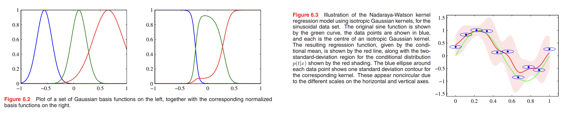
Nadaraya-Watson model
Recall the prediction of a linear regression model for a new input $\pmb{x}$ takes the form of a linear combination of the training set target values with coefficients given by the ‘equivalent kernel’ (3.62) where the equivalent kernel satisfies the summation constraint (3.64).
Gaussian Processes
In the Gaussian process viewpoint, we dispense with the parametric model and instead define a prior probability distribution over functions directly.
Linear regression revisited
Recall what we learned from linear regression
$$
y(\pmb{x}) = \pmb{w}^T \phi(\pmb{x})
\tag{6.49}
$$
when we introduce a prior distribution over $\pmb{w}$ given by an isotropic Gaussian of the form
$$
p(\pmb{w}) = N(\pmb{w} | \pmb{0}, \alpha^{-1}\pmb{I})
\tag{6.50}
$$
The probability distribution over $\pmb{w}$ defined by (6.50) therefore induces a probability distribution over functions $y(\pmb{x})$.
$$
\pmb{y} = \pmb{\Phi w}
\tag{6.51}
$$
where $\pmb{y}$ have elements $y_n = y(\pmb{x_n})$ for $n = 1, \cdots, N$, $\pmb{\Phi}$ is the design matrix with elements $\Phi_{nk} = \phi_k(\pmb{x_n})$
$\pmb{y}$ is itself Gaussian, the mean and covariance are
$$
E[\pmb{y}] = \pmb{\Phi}E[\pmb{w}] = \pmb{0}
\tag{6.52}
$$
$$
\begin{aligned}
cov[\pmb{y}] &= E[\pmb{yy^T}]\\
&= \pmb{\Phi} E[\pmb{ww^T}] \pmb{\Phi}^T \\
&= \frac{1}{\alpha} \pmb{\Phi\Phi^T} \\
&= \pmb{K}
\end{aligned}
\tag{6.53}
$$
where $\pmb{K}$ is the Gram matrix with elements
$$
K_{nm} = k(\pmb{x_n}, \pmb{x_m}) = \frac{1}{\alpha} \phi(\pmb{x_n})^T \phi(\pmb{x_m})
\tag{6.54}
$$
and $k(\pmb{x}, \pmb{x’})$ is the kernel function.
This model provides us with a particular example of a Gaussian process. In general, a Gaussian process is defined as a probability distribution over functions $y(\pmb{x})$ such that the set of values of $y(\pmb{x})$ evaluated at an arbitrary set of points $\pmb{x_1}, \cdots , \pmb{x_N}$ jointly have a Gaussian distribution.
Gaussian processes for regression
Here we shall consider noise processes that have a Gaussian distribution, so that
$$
p(t_n | y_n) = N(t_n | y_n, \beta^{-1})
\tag{6.58}
$$
Because the noise is independent for each data point, the joint distribution of the target values $\pmb{t} = (t_1, \cdots, t_N)^T$ conditioned on the values $\pmb{y} = (y_1, \cdots, y_N)^T$ is given by an isotropic Gaussian of the form
$$
p(\pmb{t} | \pmb{y}) = N(\pmb{t} | \pmb{y}, \beta^{-1}I_N)
\tag{6.59}
$$
From the definition of a Gaussian process, the marginal distribution $p(\pmb{y})$ is given by a Gaussian whose mean is zero and whose covariance is defined by a Gram matrix $\pmb{K}$ so that
$$
p(\pmb{y}) = N(\pmb{y} | \pmb{0}, \pmb{K})
\tag{6.60}
$$
The kernel function that determines $\pmb{K}$ is typically chosen to express the property that, for points $\pmb{x_n}$ and $\pmb{x_m}$ that are similar, the corresponding values $y(\pmb{x_n})$ and $y(\pmb{x_m})$ will be more strongly correlated than for dissimilar points. Here the notion of similarity will depend on the application.
Using (2.115), we see that the marginal distribution of $\pmb{t}$ is given by
$$
p(\pmb{t}) = \int p(\pmb{t} | \pmb{y}) p(\pmb{y}) d\pmb{y} = N(\pmb{t} | \pmb{0}, \pmb{C})
\tag{6.61}
$$
where the covariance matrix $\pmb{C}$ has elements
$$
C(\pmb{x_n}, \pmb{x_m}) = k(\pmb{x_n}, \pmb{x_m}) + \beta^{-1}\sigma_{nm}
\tag{6.62}
$$
One widely used kernel function for Gaussian process regression is given by the exponential of a quadratic form,
$$
k(\pmb{x_n}, \pmb{x_m}) = \theta_0 exp \lbrace -\frac{\theta_1}{2} ||\pmb{x_n} - \pmb{x_m}||^2\rbrace + \theta_2 + \theta_3 \pmb{x_n}^T\pmb{x_m}
\tag{6.63}
$$
But remember, Our goal in regression, however, is to make predictions of the target variables for new inputs, given a set of training data. To find the conditional distribution $p(t_{N+1}|\pmb{t})$, We then apply the results from Section 2.3.1 to obtain the required conditional distribution, as illustrated in Figure 6.7.
the joint distribution over $t_1, \cdots , t_{N+1}$ will be given by
$$
p(\pmb{t_{N+1}}) = N(\pmb{t_{N+1}} | \pmb{0}, \pmb{C_{N+1}})
\tag{6.64}
$$
…
we get
$$
m(\pmb{x_{N+1}}) = \pmb{k^TC_N^{-1}t}
\tag{6.66}
$$
$$
\sigma^{\pmb{x_{N+1}}} = c - \pmb{k^TC_N^{-1}k}
\tag{6.67}
$$
where vector $\pmb{k}$ has elements $k(\pmb{x_n}, \pmb{x_{N+1}})$ for $n = 1, \cdots , N$, scalar $c = k(\pmb{x_{N+1}}, \pmb{x_{N+1}}) + \beta^{-1}$
These are the key results that define Gaussian process regression. An example of Gaussian process regression is shown in Figure 6.8.
The only restriction on the kernel function is that the covariance matrix given by (6.62) must be positive definite.
For such models, we can therefore obtain the predictive distribution either by taking a parameter space viewpoint and using the linear regression result or by taking a function space viewpoint and using the Gaussian process result.