Keywords: Vector Fields and Line Integrals, Green’s Theorem, Stokes’ Theorem, Divergence, Vector Calculus
This is the Chapter16 ReadingNotes from book Thomas Calculus 14th.
Line Integrals of Scalar Functions(标量函数的曲线积分)
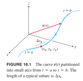
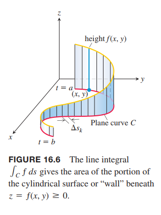
Suppose that $ƒ(x, y, z)$ is a real-valued function we wish to integrate over the curve $C$ lying within the domain of $ƒ$ and parametrized by $r(t) = g(t)i + h(t)j + k(t)k$, $a \leq t \leq b$. The values of $ƒ$ along the curve are given by the composite function $ƒ(g(t), h(t), k(t))$. We are going to integrate this composition with respect to arc length from $t = a$ to $t = b$. To begin, we first partition the curve $C$ into a finite number $n$ of subarcs (Figure 16.1). The typical subarc has length $\Delta s_k$. In each subarc we choose a point $(x_k, y_k, z_k)$ and form the sum
$$
S_n = \sum_{k=1}^n f(x_k, y_k, z_k) \Delta s_k
$$
which is similar to a 👉Riemann sum.
DEFINITION
If $ƒ$ is defined on a curve $C$ given parametrically by $r(t) = g(t)i + h(t)j + k(t)k$, $a \leq t \leq b$, then the line integral of $ƒ$ over $C$ is
$$
\int_{C}f(x,y,z)ds = \lim_{n->\infty} \sum_{k=1}^{n} f(x_k, y_k, z_k)\Delta s_k
\tag{1}
$$
provided this limit exists.
If the curve $C$ is smooth for $a \leq t \leq b$ (so $v = dr/$ is continuous and never 0) and
the function $ƒ$ is continuous on $C$, then the limit in Equation (1) can be shown to exist.
We can then apply the 👉Fundamental Theorem of Calculus >> to differentiate the 👉arc length equation >>,
$$
s(t) = \int_a^t |v(\tau)| d\tau
$$
to express $ds$ in Equation (1) as $ds = |v(t)|dt$ and evaluate the integral over $C$ as
$$
\int_C f(x,y,z) ds = \int_a^b f(g(t), h(t), k(t)) |v(t)| dt
\tag{2}
$$
How to Evaluate a Line Integral
To integrate a continuous function $ƒ(x, y, z)$ over a curve $C$:
1.Find a smooth parametrization of $C$,
$$
r(t) = g(t)i + h(t)j + k(t)k, a \leq t \leq b
$$
2.Evaluate the integral as
$$
\int_C f(x,y,z)ds = \int_a^b f(g(t), h(t), k(t)) |v(t)| dt
$$
💡For example💡:
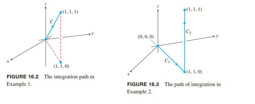
Integrate $ƒ(x, y, z) = x - 3y^2 + z$ over the line segment $C$ joining the origin to the point $(1, 1, 1)$ (Figure 16.2).
Solution:
Since any choice of parametrization will give the same answer, we choose the simplest parametrization we can think of:
$$
r(t) = ti + tj + tk, 0 \leq t \leq 1
$$
The components have continuous first derivatives and
$$
|v(t)| = |i + j + k| = \sqrt{1^2 + 1^2 + 1^2} = \sqrt{3}
$$
is never 0, so the parametrization is smooth. The integral of ƒ over $C$ is
$$
\int_C f(x,y,z)ds = \int_0^1 f(t,t,t)\sqrt{3}dt = 0
$$
Additivity
$$
\int_C f ds = \int_{C_{1}} f ds + \cdots + \int_{C_{n}} f ds
\tag{3}
$$
💡For example💡:
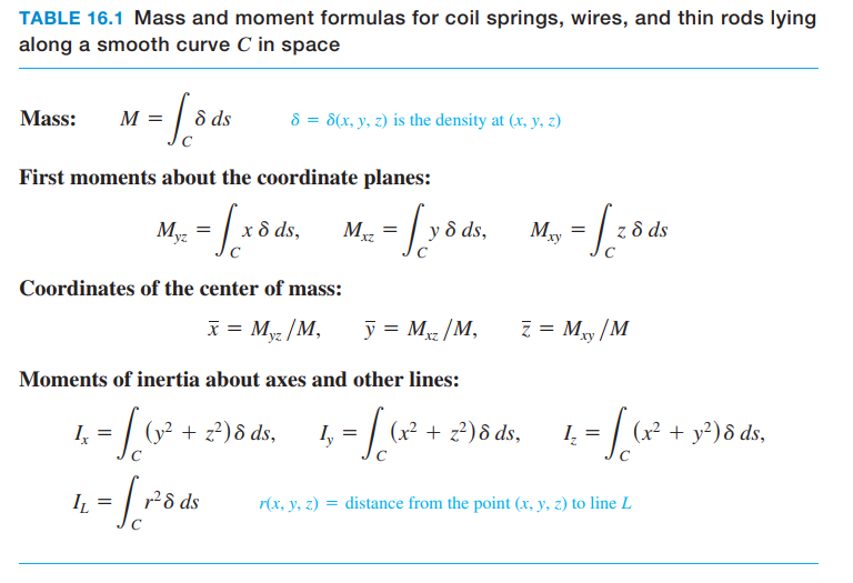
Figure 16.3 shows another path from the origin to $(1, 1, 1)$, formed from two line segments $C_1 and C_2$. Integrate $ƒ(x, y, z) = x - 3y2 + z$ over $C_1 \cup C_2$.
Solution:
$$
C_1 : r(t) = ti + tj, 0 \leq t \leq 1; |v| = \sqrt{1^2 + 1^2} = \sqrt{2}
$$
$$
C_1 : r(t) = i + j + tk, 0 \leq t \leq 1; |v| = \sqrt{0^2 + 0^2 + 1^2} = 1
$$
With these parametrizations we find that
$$
\begin{aligned}
\int_{C_1 \cup C_2} f(x,y,z) ds &= \int_{C_1} f(x,y,z) ds + \int_{C_2} f(x,y,z) ds \\
&= \int_0^1f(t,t,0) \sqrt{2}dt + \int_0^1f(1,1,t)1dt\\
&= -\frac{\sqrt{2}}{2} - \frac{3}{2}
\end{aligned}
$$
The value of the line integral along a path joining two points can change if you change the path between them.
Mass and Moment Calculations
We treat coil springs and wires as masses distributed along smooth curves in space. The distribution is described by a continuous density function $d(x, y, z)$ representing mass per unit length.
💡For example💡:
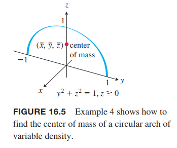
A slender metal arch, denser at the bottom than top, lies along the semicircle $y^2 + z^2 = 1, z \geq 0$, in the $yz$-plane (Figure 16.5). Find the center of the arch’s mass if the density at the point $(x, y, z)$ on the arch is $d(x, y, z) = 2 - z$.
Solution:
We know that $\bar{x} = 0$ and $\bar{y} = 0$ because the arch lies in the $yz$-plane with its mass distributed symmetrically about the $z$-axis. To find $\bar{z}$, we parametrize the circle as
$$
r(t) = (\cos t)j + (\sin t)k, 0 \leq t \leq \pi
$$
For this parametrization,
$$
|v(t)| = \sqrt{(\frac{dx}{dt})^2 + (\frac{dy}{dt})^2 + (\frac{dz}{dt})^2} = 1
$$
so $ds = |v|dt = dt$.
Thus,
$$
M = \int_C \delta ds = \int_C (2-z) ds = \int_0^\pi (2-\sin t) dt = 2\pi-2
$$
$$
M_{xy} = \int_C z\delta ds = \frac{8-\pi}{2}
$$
$$
\bar{z} = \frac{M_{xy}}{M} \approx 0.57
$$
Line Integrals in the Plane
$$
\int_C f ds = \lim_{n->\infty} \sum_{k=1}^nf(x_k,y_k)\Delta s_k
$$
Vector Fields and Line Integrals: Work, Circulation, and Flux
Just too lazy to add vector symbols while writing fomulas…
Make sure you know which is a scalar function and which is a vector function..
Vector Fields(向量场)
a vector field is a function that assigns a vector to each point in its domain. A vector field on a three-dimensional domain in space might have a formula like
$$
\vec{F}(x,y,z) = M(x,y,z)i + N(x,y,z)j+P(x,y,z)k
$$
The vector field is continuous if the component functions $M, N$, and $P$ are continuous; it is differentiable if each of the component functions is differentiable.
The formula for a field of two-dimensional vectors could look like
$$
\vec{F}(x,y) = M(x,y)i + N(x,y)j
$$
Recall what we leanred in Chapter13? The tangent vectors $T$ and normal vectors $N$ for a curve in space both form vector fields along the curve. Along a curve $r(t)$ they might have a component formula similar to the velocity field expression
$$
v(t) = f(t)i+g(t)j+h(t)k
$$
👉Vector Functions Tangents, Normals in Curve >>
Gradient Fields(梯度场)
👉More about Gradient Vectors and Several-Variables Functions >>
The gradient vector of a differentiable scalar-valued function at a point gives the direction of greatest increase of the function.
We define the gradient field of a differentiable function $ƒ(x, y, z)$ to be the field of gradient vectors
$$
\nabla f = \frac{\partial f}{\partial x} i + \frac{\partial f}{\partial y} i + \frac{\partial f}{\partial z} i
$$
At each point $(x, y, z)$, the gradient field gives a vector pointing in the direction of greatest increase of $ƒ$, with magnitude being the value of the directional derivative in that direction.(注意,梯度是向量,方向导数是标量)
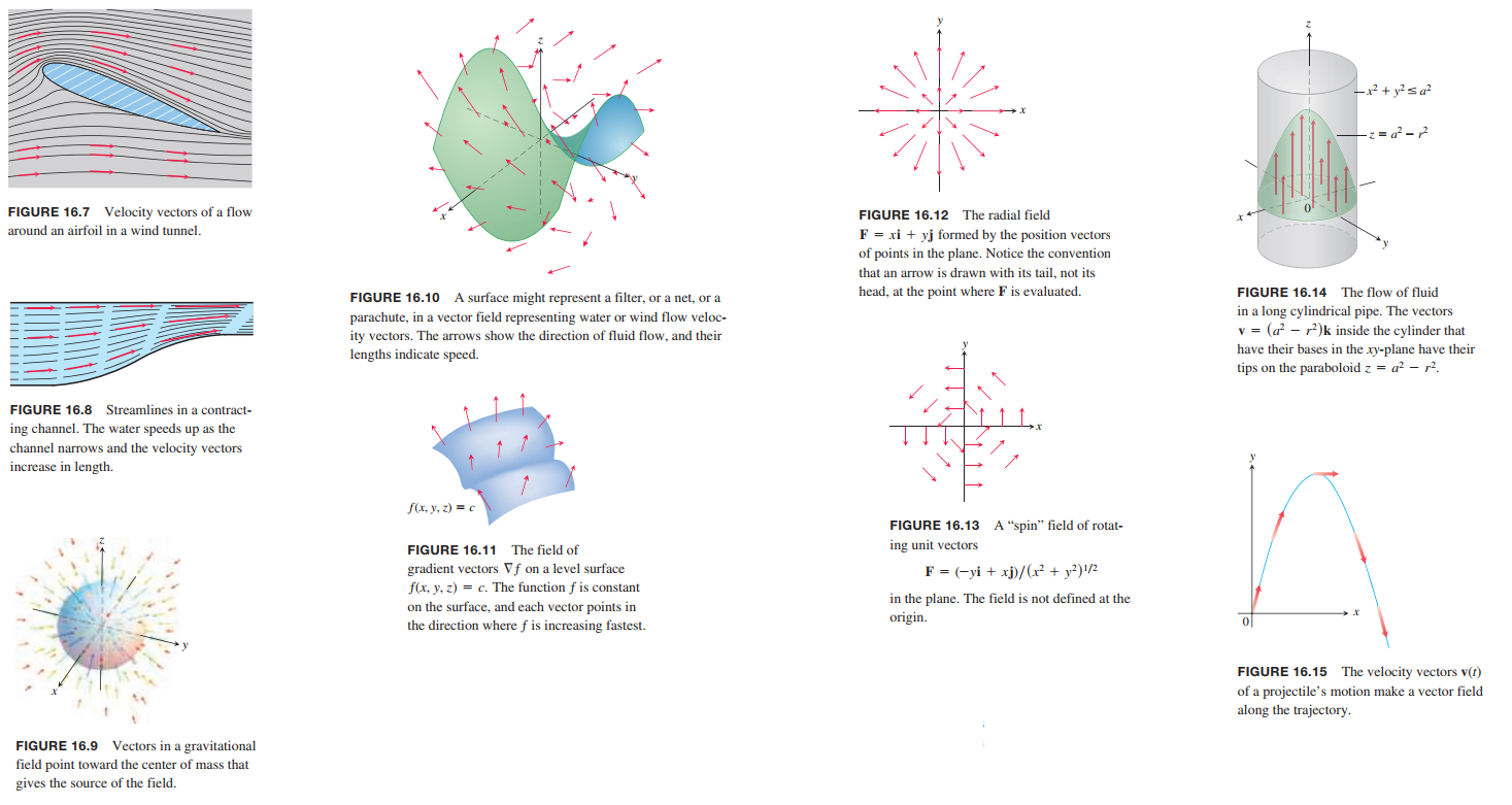
In many physical applications, $ƒ$ represents a potential energy, and the gradient vector field indicates the corresponding force. In such situations, $ƒ$ is often taken to be negative, so that the force gives the direction of decreasing potential energy.
💡For example💡:
Suppose that a material is heated, that the resulting temperature $T$ at each point $(x, y, z)$ in a region of space is given by
$$
T = 100 - x^2 - y^2 - z^2,
$$
and that $\vec{F}(x, y, z)$ is defined to be the gradient of $T$. Find the vector field $\vec{F}$.
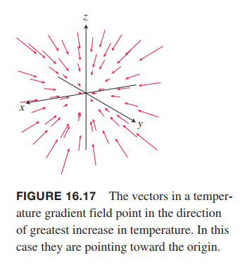
Solution:
The gradient field $F$ is the field $F = \nabla T = -2x i - 2y j - 2z k$.
Line Integrals of Vector Fields(向量场(函数)的曲线积分)
The line integral of the vector field is the line integral of the scalar tangential component of $\vec{F}$ along $C$. This tangential component is given by the dot product
$$
\vec{F} \cdot \vec{T} = \vec{F} \cdot \frac{d\vec{r}}{ds}
$$
where,
$$
\vec{T} = \frac{d\vec{r}}{ds} = \frac{\vec{v}}{|\vec{v}|}, \vec{v} = \frac{d\vec{r}}{dt}
$$
DEFINITION
Let $\vec{F}$ be a vector field with continuous components defined along a smooth curve $C$ parametrized by $\vec{r}(t)$, $a \leq t \leq b$. Then the line integral of $\vec{F}$ along $C$ is
$$
\begin{aligned}
\int_C \vec{F} \cdot \vec{T} ds &= \int_C(\vec{F} \cdot \frac{d\vec{r}}{ds}) ds\\
&= \int_C \vec{F}\cdot d\vec{r}
\end{aligned}
\tag{1}
$$
Evaluating the Line Integral of $\vec{F} = M i + N j + Pk$ Along $C: \vec{r}(t) = g(t)i + h(t) j + k(t)k$
- Express the vector field $F$ along the parametrized curve $C$ as $F(r(t))$ by substituting the components $x = g(t), y = h(t), z = k(t)$ of r into the scalar components $M(x,y,z), N(x,y,z), P(x,y,z)$ of F.
- Find the derivative (velocity) vector $dr/dt$.
- Evaluate the line integral with respect to the parameter $t$, $a \leq t \leq b$, to obtain
$$
\int_C \vec{F} \cdot d\vec{r} = \int_a^b F(r(t)) \cdot \frac{dr}{dt}dt
$$
💡For example💡:
Evaluate $\int_C \vec{F} \cdot d\vec{r}$, where $F(x, y, z) = z i + xy j - y^2 k$ along the curve $C$ given by $r(t) = t^2 i + t j + \sqrt{t} k$, $0 \leq t \leq 1$ and shown in Figure 16.18.
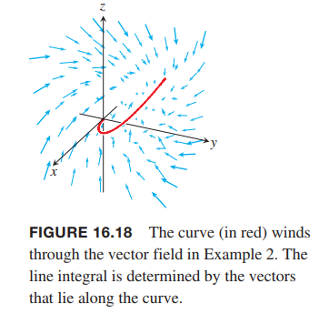
Solution:
$$
F(r(t)) = \sqrt{t}i + t^3j-t^2k
$$
$$
\frac{dr}{dt} = 2ti + j + \frac{1}{2\sqrt{t}}k
$$
Thus,
$$
\int_C F \cdot dr = \int_0^1 (2t^{3/2} + t^3 - \frac{1}{2}t^{3/2})dt = \frac{17}{20}
$$
Line Integrals with Respect to $dx, dy$, or $dz$
$$
\int_C M(x,y,z)dx = \int_C \vec{F} \cdot d\vec{r}, where, \vec{F} = M(x,y,z)i.
$$
$$
\int_C M(x,y,z)dx = \int_a^b M(g(t),h(t),k(t))g’(t)dt\tag{3}
$$
$$
\int_C N(x,y,z)dy = \int_a^b N(g(t),h(t),k(t))h’(t)dt\tag{4}
$$
$$
\int_C P(x,y,z)dz = \int_a^b P(g(t),h(t),k(t))k’(t)dt\tag{5}
$$
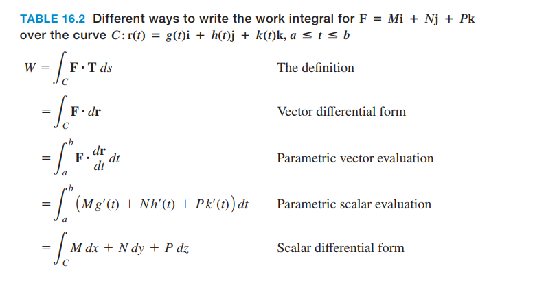
Work Done by a Force over a Curve in Space
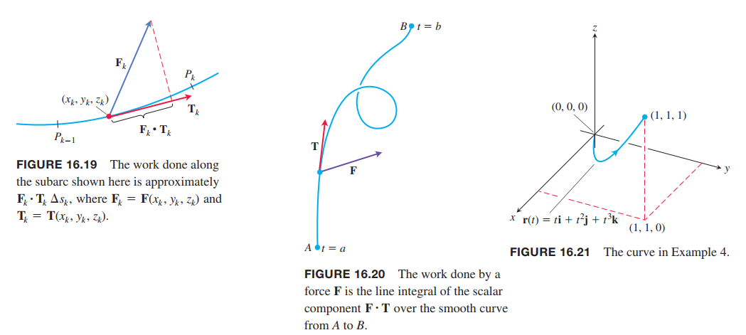
We can approximate the work as
$$
W \approx \sum_{k=1}^n W_k \approx \sum_{k=1}^n F(x_k, y_k, z_k) \cdot T(x_k, y_k, z_k) \Delta s_k
$$
as $n\rightarrow \infty$ and $\Delta s_k \rightarrow 0$, these sums approach the line integral
$$
\int_C F\cdot T ds
$$
DEFINITION
Let $C$ be a smooth curve parametrized by $r(t)$, $a \leq t \leq b$, and let $F$ be a continuous force field over a region containing $C$. Then the work done in moving an object from the point $A = r(a)$ to the point $B = r(b)$ along $C$ is
$$
W = \int_C F \cdot T ds = \int_a^b F(r(t)) \cdot \frac{dr}{dt}dt
\tag{6}
$$
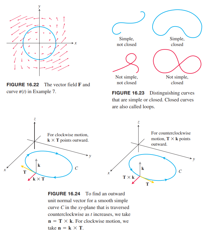
💡For example💡:
Find the work done by the force field $F = (y - x^2)i + (z - y^2)j + (x - z^2)k$ in moving an object along the curve $r(t) = t i + t^2j + t^3k$, $0 \leq t \leq 1$, from $(0, 0, 0)$ to $(1, 1, 1)$ (Figure 16.21).
Solution:
$$
F = (t^3 - t^4) j + (t - t^6)k
$$
$$
\frac{dr}{dt} = i + 2t j + 3t^2 k
$$
$$
work = \int_a^b F \cdot \frac{dr}{dt} dt = \frac{29}{60}
$$
Flow Integrals and Circulation for Velocity Fields(速度场的流量积分和循环)
DEFINITION
If $r(t)$ parametrizes a smooth curve $C$ in the domain of a continuous velocity field $F$, the flow along the curve from $A = r(a)$ to $B = r(b)$ is
$$
Flow = \int_C F \cdot T ds
\tag{7}
$$
The integral is called a flow integral. If the curve starts and ends at the same point, so that $A = B$, the flow is called the circulation around the curve.
Flux Across a Simple Closed Plane Curve(简单封闭平面曲线上的通量)
When a curve starts and ends at the same point, it is a closed curve or loop.
DEFINITION
If $C$ is a smooth simple closed curve in the domain of a continuous vector field $F = M(x, y)i + N(x, y)j$ in the plane, and if $n$ is the outwardpointing unit normal vector on $C$, the flux of $F$ across $C$ is
$$
Flux-of-F-across-C = \int_C F \cdot n ds
\tag{8}
$$
Notice the difference between flux and circulation.
$$
n = T \times k = (\frac{dx}{ds}i + \frac{dy}{ds}j) \times k = \frac{dy}{ds}i-\frac{dx}{ds}j
$$
$$
F \cdot n = M(x,y)\frac{dy}{ds} - N(x,y)\frac{dx}{ds}
$$
Hence,
$$
\int_C F \cdot n ds = \int_C (M(x,y)\frac{dy}{ds} - N(x,y)\frac{dx}{ds}) ds = \oint_C Mdy - Ndx
$$
We put a directed circle $\oint$ on the last integral as a reminder that the integration around the closed curve $C$ is to be in the counterclockwise direction.
Calculating Flux Across a Smooth Closed Plane Curve
$$
Flux-of-F = Mi + Nj \space across \space C =\oint Mdy - Ndx
\tag{9}
$$
The integral can be evaluated from any smooth parametrization $x = g(t), y = h(t), a \leq t \leq b$, that traces $C$ counterclockwise exactly once.
Path Independence, Conservative Fields, and Potential Functions
Path Independence
DEFINITIONS
Let $F$ be a vector field defined on an open region $D$ in space, and suppose that for any two points $A$ and $B$ in $D$ the line integral $\int_C F \cdot dr$ along a path $C$ from $A$ to $B$ in $D$ is the same over all paths from $A$ to $B$. Then the integral $\int_C F \cdot dr$ is path independent in $D$ and the field $F$ is conservative on $D$.
Sometimes we write $\int_C$ as $\int_A^B$ if it’s conservative.
DEFINITION
If $F$ is a vector field defined on $D$ and $F = \nabla ƒ$ for some scalar function $ƒ$ on $D$, then $ƒ$ is called a potential function(势函数) for $F$.
A gravitational potential is a scalar function whose gradient field is a gravitational field, an electric potential is a scalar function whose gradient field is an electric field, and
so on.
we can evaluate all the line integrals in the domain of $F$ over any path between $A$ and $B$ by
$$
\int_A^B F \cdot dr = \int_A^B \nabla f \cdot dr = f(B) - f(A)
\tag{1}
$$
If you think of $\nabla f$ for functions of several variables as analogous to the derivative ƒ’ for functions of a single variable
Similar to $\int_a^b f’(x) dx = f(b) - f(a)$ right?
Assumptions on Curves, Vector Fields, and Domains
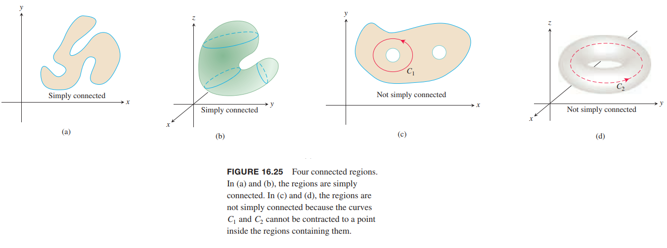
The domains $D$ we consider are connected. For an open region, this means that any two points in $D$ can be joined by a smooth curve that lies in the region. Some results require $D$ to be simply connected, which means that every loop in $D$ can be contracted to a point in $D$ without ever leaving $D$.
Line Integrals in Conservative Fields
THEOREM 1—Fundamental Theorem of Line Integrals
Let $C$ be a smooth curve joining the point $A$ to the point $B$ in the plane or in space and parametrized by $r(t)$. Let $ƒ$ be a differentiable function with a continuous vector $F = \nablaƒ$ on a domain $D$ containing $C$. Then
$$
\int_C F \cdot dr = f(B) - f(A)
$$
THEOREM 2—Conservative Fields are Gradient Fields
$F = Mi + Nj + Pk$ be a vector field whose components are continuous throughout an open connected region $D$ in space. Then $F$ is conservative if and only if $F$ is a gradient field $\nabla ƒ$ for a differentiable function $ƒ$.
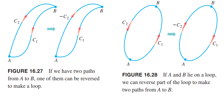
THEOREM 3—Loop Property of Conservative Fields
The following statements are equivalent.
- $\oint_C F \cdot dr = 0$ around every loop (that is, closed curve $C$ ) in $D$.
- The field $F$ is conservative on $D$.
Finding Potentials for Conservative Fields
Component Test for Conservative Fields
Let $F = M(x, y, z)i + N(x, y, z)j + P(x, y, z)k$ be a field on an open simply connected domain whose component functions have continuous first partial derivatives. Then, $F$ is conservative if and only if
$$
\frac{\partial P}{\partial y} = \frac{\partial N}{\partial z},\\
\frac{\partial M}{\partial z} = \frac{\partial P}{\partial x},\\
\frac{\partial N}{\partial x} = \frac{\partial M}{\partial y},
\tag{2}
$$

