Keywords: Second-Order Linear Equations, Euler Equations, Nonhomogeneous Linear Equations
This is the Chapter17 ReadingNotes from book Thomas Calculus 14th.
👉First-Order Differential Equations >>
Second-Order Linear Equations
An equation of the form
$$
P(x)y’’(x) + Q(x)y’(x) + R(x)y(x) = G(x)
\tag{1}
$$
which is linear in $y$ and its derivatives, is called a second-order linear differential equation.
If $G(x)$ is identically zero on $I$, the equation is said to be homogeneous; otherwise it is called nonhomogeneous.
Thus, the form of a second-order linear homogeneous differential equation is
$$
P(x)y’’ + Q(x)y’ + R(x)y = 0
\tag{2}
$$
We assume that the functions $P, Q, R$, and $G$ are continuous throughout some open interval $I$. We also assume that $P(x)$ is never zero for any $x \in I$.
THEOREM 1—The Superposition Principle
If $y_1(x)$ and $y_2(x)$ are two solutions to the linear homogeneous equation (2), then for any constants $c_1$ and $c_2$, the function
$$
y(x) = c_1y_1(x) + c_2y_2(x)
$$
is also a solution to Equation (2).
THEOREM 2
If $P, Q$, and $R$ are continuous over the open interval $I$ and $P(x)$ is never zero on $I$, then the linear homogeneous equation (2) has two linearly independent solutions $y_1$ and $y_2$ on $I$. Moreover, if $y_1$ and $y_2$ are any two linearly independent solutions of Equation (2), then the general solution is given by
$$
y(x) = c_1y_1(x) + c_2y_2(x)
$$
where $c_1$ and $c_2$ are arbitrary constants.
Constant-Coefficient Homogeneous Equations
Suppose we wish to solve the second-order homogeneous differential equation
$$
ay’’ + by’ + c = 0
\tag{3}
$$
where $a, b$, and $c$ are constants.
If we substitute $y = e^{rx}$ into Equation (3), we obtain
$$
ar^2e^{rx} + bre^{rx} + ce^{rx} = x_0
$$
$y = e^{rx}$ is a solution to Equation (3) if and only if $r$ is a solution to the auxiliary equation (or characteristic equation)
$$
ar^2 + br + c = 0\tag{4}
$$
the roots are
$$
r_1 = \frac{-b + \sqrt{b^2-4ac}}{2a}and r_2 = \frac{-b - \sqrt{b^2-4ac}}{2a}
$$
Case1: $b^2-4ac > 0$
THEOREM 3
If $r_1$ and $r_2$ are two real and unequal roots to the auxiliary equation(辅助方程) $ar^2 + br + c = 0$, then
$$
y = c_1 e^{r_1 x} + c_2 e^{r_2 x}
$$
is the general solution to $ay’’ + by’ + cy = 0$.
Case2: $b^2-4ac = 0$
THEOREM 4
If $r$ is the only(repeated) root to the auxiliary equation(辅助方程) $ar^2 + br + c = 0$, then
$$
y = c_1 e^{r x} + c_2 x e^{rx}
$$
is the general solution to $ay’’ + by’ + cy = 0$.
Case3: $b^2-4ac < 0$
THEOREM 5
If $r_1 = \alpha + i\beta$ and $r_2 = \alpha - i\beta$ are two complex roots to the auxiliary equation $ar^2 + br + c = 0$, then
$$
y = e^{\alpha x}(c_1\cos\beta x + c_2 \sin \beta x)
$$
is the general solution to $ay’’ + by’ + cy = 0$.
$\alpha = -b/2a, and ,\beta = \sqrt{4ac-b^2}/2a$
Initial Value and Boundary Value Problems
THEOREM 6
If $P, Q, R$, and $G$ are continuous throughout an open interval $I$, then there exists one and only one function $y(x)$ satisfying both the differential equation
$$
P(x)y’’(x) + Q(x)y’(x) + R(x)y(x) = G(x)
$$
on the interval $I$, and the initial conditions
$$
y(x_0) = y_0, and, y’(x_0) = y_1
$$
at the specified point $x \in I$.
Another approach to get a unique solution is boundary values,
$$
y(x_1) = y_1 ,and, y(x_2) = x_2
$$
The differential equation together with specified boundary values is called a boundary value problem.
Nonhomogeneous Linear Equations
Form of the General Solution
Suppose we wish to solve the nonhomogeneous equation
$$
ay’’+by’+cy = G(x)
\tag{1}
$$
where $a, b$, and $c$ are constants and $G$ is continuous over some open interval $I$.
Let $y_c = c_1y_1 + c_2y_2$ be the general solution to the associated complementary equation(互补方程)
$$
ay’’+by’+c = 0
\tag{2}
$$
Now suppose we could somehow come up with a particular function $y_p$ that solves the nonhomogeneous equation (1).
$$
y = y_c + y_p
\tag{3}
$$
THEOREM 7
The general solution $y = y(x)$ to the nonhomogeneous differential equation (1) has the form
$$
y = y_c + y_p
$$
where the complementary solution $y_c$ is the general solution to the associated homogeneous equation (2) and $y_p$ is any particular solution to the nonhomogeneous equation (1).
Recall what we have learned in Linear Algebra. The relationship between $Ax = 0$ and $Ax = b$?
👉Homegenous and Nonhomegenous in Algebra >>
The Method of Undetermined Coefficients(待定系数法)
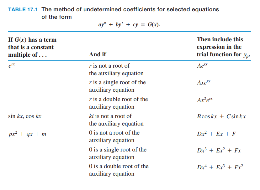
💡For example💡:
Solve the nonhomogeneous equation $y’’-2y’-3y = 1-x^2$.
Solution:
auxiliary equation for the complementary equation $y’’-2y’-3y = 0$ is
$$
r^2 - 2r -3 = 0 \rightarrow (r+1)(r-3) = 0
$$
the complementary solution
$$
y_c = c_1 e^{-x} + c_2 e^{3x}
$$
Now $G(x) = 1 - x^2$ is a polynomial of degree $2$. It would be reasonable to assume that a particular solution to the given nonhomogeneous equation is also a polynomial of degree $2$.
$$
y_p = Ax^2 + Bx + C
$$
substitute $y_p$ to the original equation, we get
$$
-3Ax^2 + (-4A-3B)x + (2A-2B-3C) = 1-x^2
$$
thus, we get
$$
\begin{cases}
-3A = -1\\
-4A - 3B = 0\\
2A-3B-3C = 1
\end{cases}
$$
so that,
$$
y = y_c + y_p = c_1 e^{-x} + c_2 e^{3x} + \frac{1}{3}x^2 - \frac{4}{9}x + \frac{5}{27}
$$
The Method of Variation of Parameters(参数变分法)
Assume $c_1$ and $c_2$ are two functions $v_1$ and $v_2$.
Then, First, the complementary solution $y = v_1y_1 + v_2y_2$ should satisfy Equation(1).Second,
$$
v_1’y_1 + v_2’y_2 = 0
\tag{4}
$$
Thus, we have
$$
v_1(ay_1’’ + by_1’ + cy_1) + v_2(ay_2’’ + by_2’ + cy_2) + a(v_1’y_1’ + v_2’y_2’) = G(x)
$$
the first two terms are zero. so
$$
a(v_1’ y_1’ + v_2’y_2’) = G(x)
\tag{5}
$$
Variation of Parameters Procedure
To use the method of variation of parameters to find a particular solution(特解) to the nonhomogeneous equation
$$
ay’’ + by’ + cy = G(x)
$$
we can work directly with Equations (4) and (5). It is not necessary to rederive them. The steps are as follows.
- Solve the associated homogeneous equation
$$
ay’’+by’+c = 0
$$
to find the functions $y_1$ and $y_2$.- Solve the equations
$$
v_1’y_1 + v_2’y_2 = 0,\\
v_1’y_1’+v_2’y_2’ = \frac{G(x)}{a}
$$
simultaneously for the derivative functions $v’_1$ and $v’_2$. (method of determinants (also known as Cramer’s Rule))- Integrate $v’_1$ and $v’_2$ to find the functions $v_1 = v_1(x)$ and $v_2 = v_2(x)$.
- Write down the particular solution to nonhomogeneous equation (1) as
$$
y_p = v_1y_1 + v_2y_2
$$
💡For example💡:
Find the general solution to the equation
$$
y’’+y = \tan x
$$
Solution:
The solution of the homogeneous equation
$$
y’’ + y = 0
$$
is given by
$$
y_c = c_1 \cos x + c_2 \sin x
$$
Since $y_1(x) = \cos x$ and $y_2(x) = \sin x$, the conditions to be satisfied in Equations (4) and (5) are
$$
\begin{cases}
v_1’ \cos x + v_2’ \sin x = 0\\
-v_1’ \sin x + v_2’ \cos x = \tan x, a = 1
\end{cases}
$$
Solution of this system gives
$$
v_1’ = \frac{\left | \begin{matrix}
0 & \sin x\\
\tan x & \cos x
\end{matrix}\right |}{\left | \begin{matrix}
\cos x & \sin x\\
-\sin x & \cos x
\end{matrix}\right |}
=
\frac{-\sin^2 x}{\cos x}
$$
$$
v_2’ = \frac{\left | \begin{matrix}
\cos x & 0\\
-\sin x & \tan x
\end{matrix}\right |}{\left | \begin{matrix}
\cos x & \sin x\\
-\sin x & \cos x
\end{matrix}\right |}
=
\sin x
$$
After integrating $v’_1$ and $v’_2$, we have
$$
v_1(x) = \int \frac{-\sin^2 x}{\cos x} dx
=-\ln |\sec x + \tan x| + \sin x
$$
and
$$
v_2(x) = \int \sin x dx = -\cos x
$$
Thus,
$$
y_p = (-\cos x)\ln|\sec x + \tan x|
$$
thus,
$$
y = c_1 \cos x + c_2 \sin x -\cos x\ln|\sec x + \tan x|
$$
Applications
Vibrations(振动)
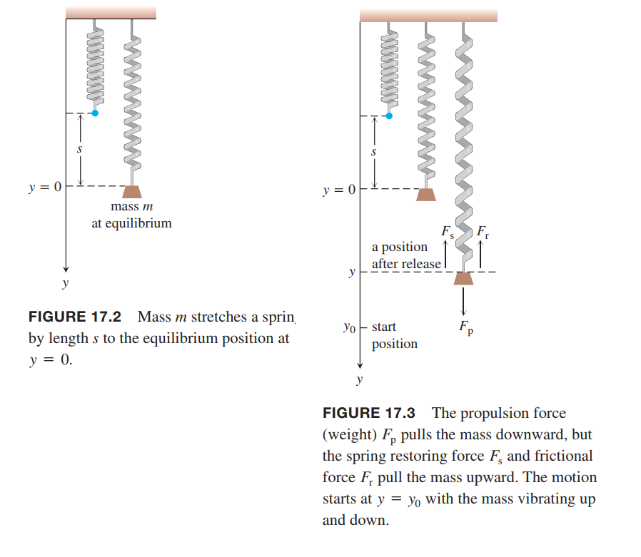
See Figure 17.2, according Hooke’s Law, equilibrium requires that
$$
ks = mg
\tag{1}
$$
Suppose that the object is pulled down an additional amount $y_0$ beyond the equilibrium position and then released.
Then the forces acting on the object are:
the propulsion force due to gravity(由重力引起的推进力),
$$
F_p = mg
$$
the restoring force of the spring’s tension(弹簧张力的恢复力),
$$
F_s = k(s+y)
$$
a frictional force assumed proportional to velocity(和速度成正比的摩擦力),
$$
F_r = \delta \frac{dy}{dt}
$$
By Newton’s second law $F = ma$,
$$
m \frac{d^2y}{d^2t} = mg - ks - ky - \delta \frac{dy}{dt}
$$
By Equation (1), $mg - ks = 0$, then
$$
m \frac{d^2y}{d^2t} + \delta \frac{dy}{dt} + ky = 0
\tag{2}
$$
subject to the initial conditions $y(0) = y_0$ and $y’(0) = 0$.
The motion is: motion predicted by Equation (2) will be oscillatory about the equilibrium position $y = 0$ and eventually damp to zero because of the retarding frictional force.
Simple Harmonic Motion(简谐运动)
Suppose no frictional force. $\delta = 0$ and there is no damping.
We substitude $\omega = \sqrt{k/m}$ to simplify our calculations.
Then equation(2) becomes,
$$
y’’ + \omega ^2 y = 0, with, y(0) = y_0, y’(0) = 0
$$
The general solution is
$$
y = c_1 \cos \omega t + c_2 \sin \omega t
\tag{3}
$$
The particular solution is
$$
y = y_0 \cos \omega t
\tag{4}
$$
Equation (4) represents simple harmonic motion of amplitude $y_0$ and period $T = 2\pi / \omega$.
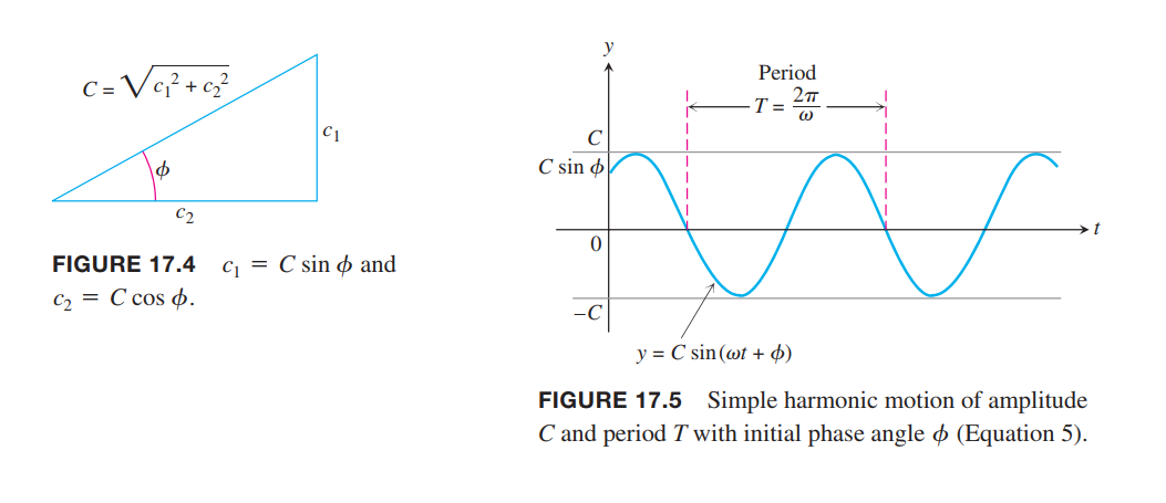
The general solution given by Equation (3) can be combined into a single term by using the trigonometric identity(使用三角恒等式)
$$
\sin(\omega t + \phi) = \cos \omega t \sin \phi + \sin \omega t \cos \phi
$$
so that
$$
c_1 = C\sin \phi, c_2 = C\cos \phi
$$
where
$$
C = \sqrt {c_1^2 + c_2^2}, \phi = \tan^{-1} \frac{c_1}{c_2}
$$
Then the general solution in Equation (3) can be written in the alternative form
$$
y = C \sin (\omega t + \phi)
\tag{5}
$$
The angle $\omega t + \phi$ is called the phase angle(相位角), and $\phi$ may be interpreted as its initial value.
A graph of the simple harmonic motion represented by Equation (5) is given in Figure 17.5.
Damped Motion(阻尼运动)
Assume now that there is friction in the spring system, so $\delta \neq 0$.
$$
\omega = \sqrt{k/m}, 2b = \delta / m
$$
then the differential equation (2) is
$$
y’’ + 2by’ + \omega^2 y = 0
\tag{6}
$$
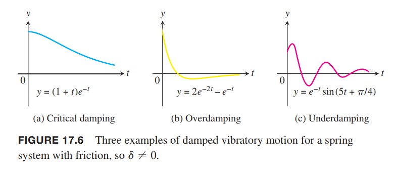
Obviously the auxiliary equation of (6) is
$$
r^ 2 + 2br + \omega^2 = 0
$$
the root $r = -b \pm \sqrt{b^2-\omega^2}$
Case1. $b = \omega$ The general solution is
$$
y = (c_1 + c_2t)e^{-\omega t}
$$
This situation of motion is called critical damping and is not oscillatory(临界阻尼,不振荡).
Case2. $b > \omega$ The general solution is
$$
y = c_1e^{(-b+\sqrt{b^2-\omega^2})t} + c_2e^{(-b-\sqrt{b^2-\omega^2})t}
$$
Here again the motion is not oscillatory and both $r_1$ and $r_2$ are negative. Thus $y$ approaches zero as time goes on. This motion is referred to as overdamping(过阻尼,不振荡).
Case3. $b < \omega$ The general solution is
$$
y = e^{-bt}(c_1\cos \sqrt{\omega^2-b^2}t + c_2\sin \sqrt{\omega^2-b^2}t)
$$
This situation, called underdamping(欠阻尼), represents damped oscillatory motion. It is analogous to simple harmonic motion of period $T = 2\pi/ \sqrt{\omega^2 - b^2}$ except that the amplitude is not constant but damped by the factor $e^{-bt}$.
Therefore, the motion tends to zero as $t$ increases, so the vibrations tend to die out as time goes on. Notice that the period $T = 2\pi/ \sqrt{\omega^2 - b^2}$ is larger than the period $T_0 = 2\pi/ \omega$ in the friction-free system.
Moreover, the larger the value of $b = \delta / 2m$ in the exponential damping factor, the more quickly the vibrations tend to become unnoticeable. A curve illustrating underdamped motion is shown in Figure 17.6c.
Electric Circuits(电路)
to be added..
Summary
Euler Equations
Euler equations have this form
$$
P(x) = ax^2, Q(x) = bx, R(x) = c
$$
where $a, b$, and $c$ are constants.
The General Solution of Euler Equations
Consider the Euler equation
$$
ax^2 y’’ + bx y’ + cy = 0, x > 0
\tag{1}
$$
The essence is : change it into constant coefficients equation.
Let $z = \ln x$ and $y(x) = Y(z)$.
$$
\begin{aligned}
y’(x) &= \frac{d}{dx}Y(z)\\ &= \frac{d}{dz}Y(z)\frac{dz}{dx}\\ &= Y’(z)\frac{1}{x}
\end{aligned}
$$
$$
\begin{aligned}
y’’(x) &= \frac{d}{dx}y’(x)\\ &= \frac{d}{dx}Y’(z)\frac{1}{x}\\
&=-\frac{1}{x^2}Y’(z) + \frac{1}{x}Y’’(z)\frac{dz}{dx}\\
&= -\frac{1}{x^2}Y’(z) + \frac{1}{x^2}Y’’(z)
\end{aligned}
$$
thus,
$$
ax^2 y’’ + bx y’ + cy = 0 = aY’’(z) + (b-a)Y’(z) + cY(z)
$$
Now it’s changed to solve this equation:
$$
aY’’(z) + (b-a)Y’(z) + cY(z) = 0
\tag{2}
$$
we find the roots to the associated auxiliary equation
$$
ar^2 + (b-a)r + c = 0
\tag{3}
$$
💡For example💡:
Find the particular solution to $x^2y’’ - 3xy’ + 68y = 0$ that satisfies the initial conditions $y(1) = 0$ and $y’(1) = 1$.
Solution:
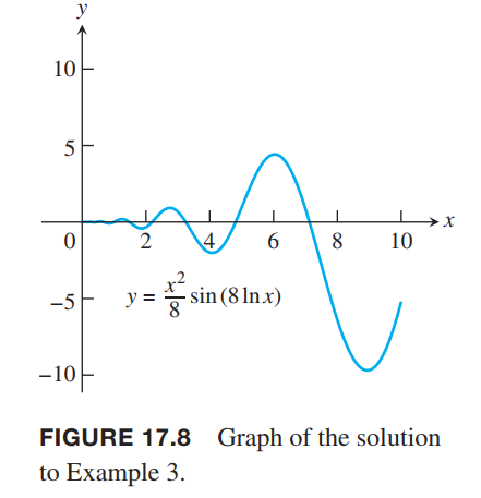
$$
Y(z) = e^{2z}(c_1\cos8z + c_2 \sin 8z)
$$
$$
y(x) = e^{2\ln x}(c_1\cos8 \ln x + c_2 \sin 8 \ln x)
$$
from the two conditions, we get
$$
c_1 = 0, c_2 = \frac{1}{8}
$$
thus,
$$
y(x) = \frac{1}{8}x^2 \sin(8\ln x), -\frac{x^2}{8} \leq y \leq \frac{x^2}{8}
$$
Power-Series Solutions
Method of Solution
The power-series method for solving a second-order homogeneous differential equation consists of finding the coefficients of a power series(幂级数)
$$
y(x) = \sum_{n=0}^{\infty}c_nx^n = c_0 + c_1 x + c_2 x^2 + \cdots
\tag{1}
$$
which solves the equation.
💡For example💡:
Solve the equation $y’’ + y = 0$ by the power-series method.
Solution:
We assume the series solution takes the form of
$$
y = \sum_{n=0}^{\infty} c_n x^n
$$
and calculate the derivatives
$$
y’ = \sum_{n=1}^{\infty} nc_nx^{n-1}
$$
and
$$
y’’ = \sum_{n=2}^{\infty}n(n-1)c_nx^{n-2}
$$
Substitution of these forms into the second-order equation gives us
$$
\sum_{n=2}^{\infty}n(n-1)c_nx^{n-2} + \sum_{n=0}^{\infty}c_nx^n = 0
$$
Next, we equate the coefficients of each power of x to zero as summarized in the following table.
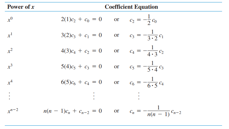
Even indices:
Here $n = 2k$, so the power is $x^{2k-2}$. we have
$$
2k(2k-1)c_{2k} + c_{2k-2} = 0
$$
or
$$
c_{2k} = -\frac{1}{2k(2k-1)}c_{2k-2}
$$
From this recursive relation we find
$$
c_{2k} = [-\frac{1}{2k(2k-1)}] \cdots [-\frac{1}{2}] c_0
=\frac{(-1)^k}{(2k)!}c_0
$$
Odd indices:
$$
(2k+1)(2k)c_{2k+1} + c_{2k-1} = 0
$$
Thus,
$$
c_{2k+1} = \frac{(-1)^k}{(2k+1)!}c_1
$$
Thus,
$$
\begin{aligned}
y &= \sum_{n=0}^{\infty} c_n x^n\\
&= \sum_{k=0}^{\infty} c_{2k}x^{2k} + \sum_{k=0}^{\infty}c_{2k+1}x^{2k+1}\\
&= c_0 \sum_{k=0}^{\infty}\frac{(-1)^k}{(2k)!}x^{2k} + c_1 \sum_{k=0}^{\infty}\frac{(-1)^k}{(2k+1)!}x^{2k+1}\\
&=c_0 \cos x + c_1 \sin x
\end{aligned}
$$

