NumericalAnalysis-C12-Eigenvalues-and-Singular-Values

Keywords: Power Iteration Method, QR Algorithm, SVD(Singular Value Decomposition), Mathlab

This is the Chapter12 ReadingNotes from book Numercial Analysis(Timothy Sauer).

👉More about EigenValues and EigenVectors in Algebra >>

Power Iteration Methods

There is no direct method for computing eigenvalues. The situation is analogous to rootfinding, in that all feasible methods depend on some type of iteration.

Power Iteration

The motivation behind Power Iteration is that multiplication by a matrix tends to move vectors toward the dominant eigenvector direction.

DEFINITION 12.1
Let $A$ be an $m × m$ matrix. A dominant eigenvalue of $A$ is an eigenvalue $\lambda$ whose magnitude is greater than all other eigenvalues of $A$. If it exists, an eigenvector associated to $\lambda$ is called a dominant eigenvector.

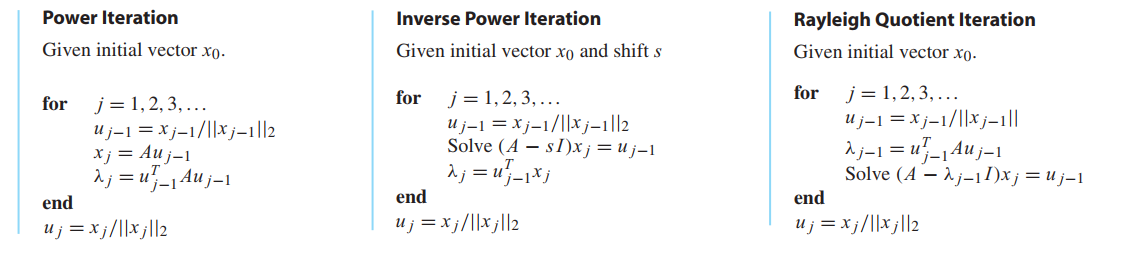
To keep the numbers from getting out of hand, it is necessary to normalize the vector at each step.

Given an approximate eigenvector, the Rayleigh quotient is the best approximate eigenvalue. (least squares, take $\lambda$ as unknows, $x$ as coefficient matrix)
$$
Ax = \lambda x \\
x\lambda = Ax\\
x^Tx\lambda = x^TAx\\
\lambda = \frac{x^TAx}{x^Tx}
\tag{12.2}
$$

1
2
3
4
5
6
7
8
9
10
11
12

%powerit.m
% Program 12.1 Power Iteration
% Computes dominant eigenvector of square matrix
% Input: matrix A, initial (nonzero) vector x, number of steps k
% Output: dominant eigenvalue lam, eigenvector u
function [lam,u]=powerit(A,x,k)
for j=1:k
    u=x/norm(x); % normalize vector
    x=A*u; % power step
    lam=u'*x; % Rayleigh quotient
end
u=x/norm(x);

Convergence of Power Iteration

THEOREM 12.2
Let $A$ be an $m \times m$ matrix with real eigenvalues $\lambda_1, \cdots, \lambda_m$ satisfying $|\lambda_1| > |\lambda_2| \geq |\lambda_3| \geq \cdots \geq |\lambda_m|$. Assume that the eigenvectors of $A$ span $R^m$. For almost every initial vector, Power Iteration converges linearly to an eigenvector associated to $\lambda_1$ with convergence rate constant $S = |\lambda_2 / \lambda_1|$.

Inverse Power Iteration

LEMMA 12.3
Let the eigenvalues of the $m \times m$ matrix A be denoted by $\lambda_1, \cdots, \lambda_m$ .
(a) The eigenvalues of the inverse matrix $A^{−1}$ are $\lambda_1^{-1}, \cdots, \lambda_m^{-1}$, assuming that the inverse exists. The eigenvectors are the same as those of $A$.
(b) The eigenvalues of the shifted matrix $A − sI$ are $\lambda_1 − s, \lambda_2 − s, \cdots,\lambda_m − s$ and the eigenvectors are the same as those of $A$.

According to Lemma 12.3, the largest magnitude eigenvalue of the matrix $A^{−1}$ is the reciprocal of the smallest magnitude eigenvalue of $A$.

$$
x_{k+1} = A^{-1}x_k \Leftrightarrow Ax_{k+1} = x_{k}
\tag{12.4}
$$
which is then solved for $x_{k+1}$ by Gaussian elimination.

Suppose $A$ has an eigenvalue 10.05, near 10, then $A-10I$ has an eigenvalue $\lambda = 0.05$. If it is the smallest magnitude eigenvalue of $A-10I$, then the inverse Power Iteration $x_{k+1} = (A-10I)^{-1}x_k$ will locate it.

That is, the Inverse Power Iteration will converge to the reciprocal $1/(.05) = 20$, after which we invert to $.05$ and add the shift back to get $10.05$.

This trick will locate the eigenvalue that is smallest after the shift—which is another way
of saying the eigenvalue nearest to the shift.

Look at the figure again.

1
2
3
4
5
6
7
8
9
10
11
12
13

%invpowerit.m
% Program 12.2 Inverse Power Iteration
% Computes eigenvalue of square matrix nearest to input s
% Input: matrix A, (nonzero) vector x, shift s, steps k
% Output: dominant eigenvalue lam, eigenvector of inv(A-sI)
function [lam,u]=invpowerit(A,x,s,k)
As=A-s*eye(size(A));
for j=1:k
    u=x/norm(x); % normalize vector
    x=As\u; % power step
    lam=u'*x; % Rayleigh Quotient
end
lam=1/lam+s; u=x/norm(x);

Rayleigh Quotient Iteration

If at any step along the way an approximate eigenvalue were known, it could be used as the shift $s$, to speed convergence.

1
2
3
4
5
6
7
8
9
10
11
12

%rqi.m
% Program 12.3 Rayleigh Quotient Iteration
% Input: matrix A, initial (nonzero) vector x, number of steps k
% Output: eigenvalue lam and eigenvector u
function [lam,u]=rqi(A,x,k)
for j=1:k
    u=x/norm(x); % normalize
    lam=u'*A*u; % Rayleigh quotient
    x=(A-lam*eye(size(A)))\u; % inverse power iteration
end
u=x/norm(x);
lam=u'*A*u; % Rayleigh quotient

QR Algorithms

The goal of this section is to develop methods for finding all eigenvalues at once.

👉More about Symmetric Matrix EigenVector and SVD in Algebra>>

Simultaneous iteration（同时迭代）

Real Schur form and the QR algorithm

Upper Hessenberg form

Singular Value Decomposition

Finding the SVD in general

LEMMA 12.10
Let $A$ be an $m \times n$ matrix. The eigenvalues of $A^TA$ are nonnegative.

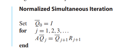
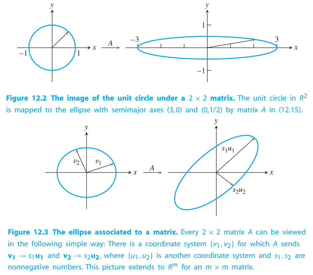
THEOREM 12.11
Let $A$ be an $m \times n$ matrix. Then there exist two orthonormal bases ${v_1, \cdots, v_n}$ of $R^n$, and ${u_1, \cdots ,u_m}$ of $R^m$, and real numbers $s_1 \geq \cdots \geq s_n \geq 0$ such that $Av_i = s_iu_i$ for $1 \leq i \leq min\lbrace m,n\rbrace$. The columns of $V = [v_1| . . . |v_n]$, the right singular vectors, are the set of orthonormal eigenvectors of $A^TA$; and the columns of $U = [u_1| \cdots |u_m]$, the left singular vectors, are the set of orthonormal eigenvectors of $AA^T$.

$$
A = \begin{bmatrix}
3 & 0\\
0 & \frac{1}{2}
\end{bmatrix}
\tag{12.15}
$$
$$
Av_1 = s_1 u_1\\
\cdots \\
Av_n = s_n u_n
\tag{12.16}
$$

Special case: symmetric matrices

Finding the SVD of a symmetric $m \times m$ matrix is simply a matter of finding the eigenvalues and eigenvectors.

Application of SVD

Properties of the SVD

Dimension reduction

Compression

Calculating the SVD