Keywords: Euler’s Method, First-order linear equations, Systems of Ordinary Differential Equations, Implicit Methods and Stiff Equations, Mathlab
👉More about First-Order-Differential-Equations in Calculus >>
👉More about Second-Order-Differential-Equations in Calculus >>
Initial Value Problems
A wide majority of interesting equations have no closed-form solution, which leaves approximations as the only recourse.
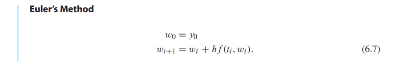
It will be helpful to think of a differential equation as a field of slopes, When an initial condition is specified on a slope field, one out of the infinite family of solutions can be identified.
Euler’s Method
💡For example💡:
draw the slope field of this initial value problem, and apply Euler’s Method to this initial value problem with initial condition $y_0 = 1$
$$
\begin{cases}
y’ = ty + t^3\\
y(0) = y_0\\
t \in [0,1]
\end{cases}
\tag{6.5}
$$
Solution:
The right-hand side of the differential equation is $f(t,y) = ty + t^3$. Therefore, Euler’s Method will be the iteration
$$
w_0 = 1\\
w_{i+1} = w_i + h(t_iw_i + t_i^3)
\tag{6.8}
$$
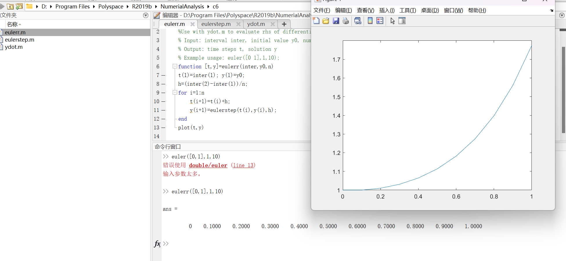
1 | %eulerr.m |
1 | %eulerstep.m |
1 | %ydot.m |
1 | >> eulerr([0,1],1,10) |
Existence, uniqueness, and continuity for solutions
DEFINITION 6.1
A function $f(t,y)$ is Lipschitz continuous(李普希兹连续) in the variable $y$ on the rectangle $S = [a,b] \times [\alpha,\beta]$ if there exists a constant $L$ (called the Lipschitz constant) satisfying
$$
|f(t,y_1) - f(t,y_2)| \leq L|y_1 - y_2|
$$
for each $(t, y_1), (t ,y_2)$ in $S$.
A function that is Lipschitz continuous in $y$ is continuous in $y$, but not necessarily differentiable.
💡For example💡:
Find the Lipschitz constant for the right-hand side
$$
f(t,y) = ty + t^3
$$
of (6.5).
Solution:
The function $f(t,y) = ty + t^3$ is Lipschitz continuous in the variable $y$ on the set $0 \leq t \leq 1, -\infty < y < +\infty$. Check that
$$
|f(t,y_1) - f(t,y_2)| = |ty_1 - ty_2| \leq |t||y_1-y_2| \leq |y_1 - y_2|
\tag{6.10}
$$
on the set. The Lipschitz constant is $L = 1$.
If the function $f$ is continuously differentiable in the variable $y$, the maximum absolute value of the partial derivative $\frac{\partial f}{\partial y}$ is a Lipschitz constant.
According to the 👉Mean Value Theorem >>, for each fixed $t$, there is a $c$ between $y_1$ and $y_2$ such that
$$
\frac{f(t,y_1) - f(t,y_2)}{y_1 - y_2} = \frac{\partial f}{\partial y}(t,c)
$$
Therefore, $L$ can be taken to be the maximum of
$$
|\frac{\partial f}{\partial y}(t,c)|
$$
on the set.
The Lipschitz continuity hypothesis guarantees the existence and uniqueness of solutions of initial value problems.
THEOREM 6.2
Assume that $f(t,y)$ is Lipschitz continuous in the variable $y$ on the set $S = [a,b] \times [\alpha,\beta]$ and that $\alpha < y_a < \beta$. Then there exists $c$ between $a$ and $b$ such that the initial value problem
$$
\begin{cases}
y’ = f(t,y)\\
y(a) = y_a\\
t \in [a,c]
\end{cases}
\tag{6.11}
$$
has exactly one solution $y(t)$.
Moreover, if $f$ is Lipschitz on $[a,b] \times [-\infty,+\infty]$, then there exists exactly one solution on $[a,b]$.
THEOREM 6.3
Assume that $f(t,y)$ is Lipschitz in the variable $y$ on the set $S = [a,b] \times [\alpha,\beta]$. If $Y(t)$ and $Z(t)$ are solutions in $S$ of the differential equation
$$
y’ = f(t,y)
$$
with initial conditions $Y(a)$ and $Z(a)$ respectively, then
$$
|Y(t) - Z(t)| \leq e^{L(t-a)} |Y(a)-Z(a)|
\tag{6.13}
$$
==hard to understand…==
First-order linear equations
$$
\begin{cases}
y’ = g(t)y+h(t)\\
y(a) = y_a\\
t \in [a,b]
\end{cases}
$$
the explicit solution:
$$
y(t) = e^{\int g(t) dt} \int e^{-\int g(t) dt} h(t) dt
\tag{6.16}
$$
Analysis of IVP Solvers
A careful investigation of error in Euler’s Method will illustrate the issues for IVP solvers in general.

