Animation-C5-Kinematic-Linkages

Keywords: Inverse kinematics, Forward kinematics, Hierarchy

This is the Chapter5 ReadingNotes from book Computer Animation_ Algorithms and Techniques_ Parent-Elsevier (2012).

This chapter is concerned with animating objects whose motion is relative to another object, especially when there is a sequence of objects where each object’s motion can easily be described relative to the previous one. Such an object sequence forms a motion hierarchy.

Often the components of the hierarchy represent objects that are physically connected and are referred to by the term linked appendages or, more simply, as linkages.

Hierarchical modeling

Hierarchical modeling is the enforcement of relative location constraints among objects organized in a treelike structure.

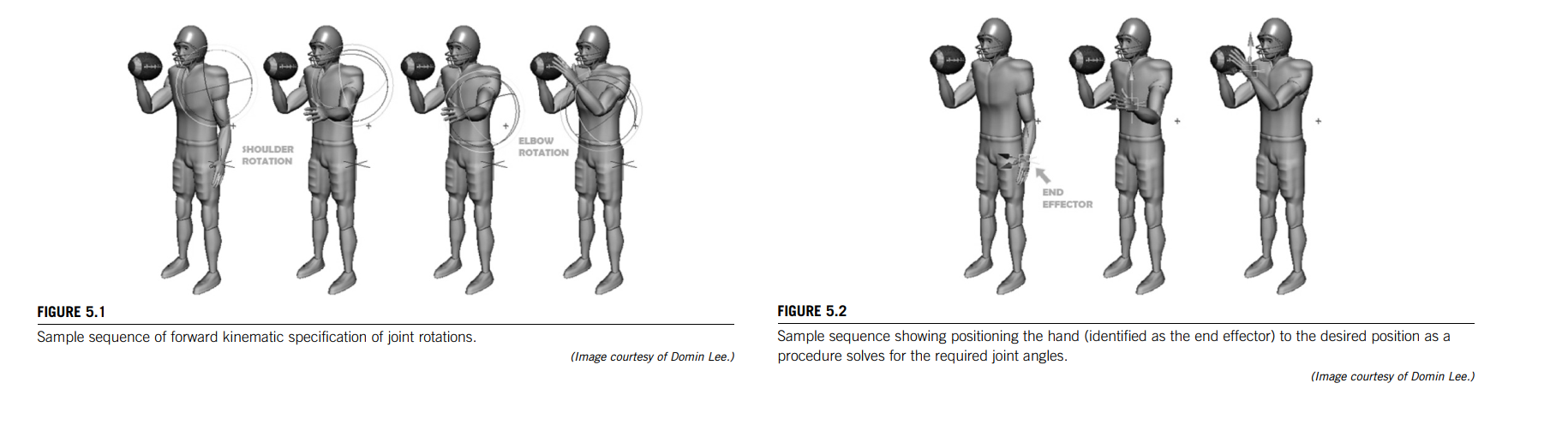
A common type of hierarchical model used in graphics has objects that are connected end to end to form multibody jointed chains. Such hierarchies are useful for modeling animals and humans so that the joints of the limbs are manipulated to produce a figure with moving appendages. Such a figure is often referred to as articulated and the movement of an appendage by changing the configuration of a joint is referred to as articulation.

The robotics literature discusses the modeling of manipulators, a sequence of objects connected in a chain by joints. The rigid objects forming the connections between the joints are called links, and the free end of the chain of alternating joints and links is called the end effector. The local coordinate system associated with each joint is referred to as the frame.

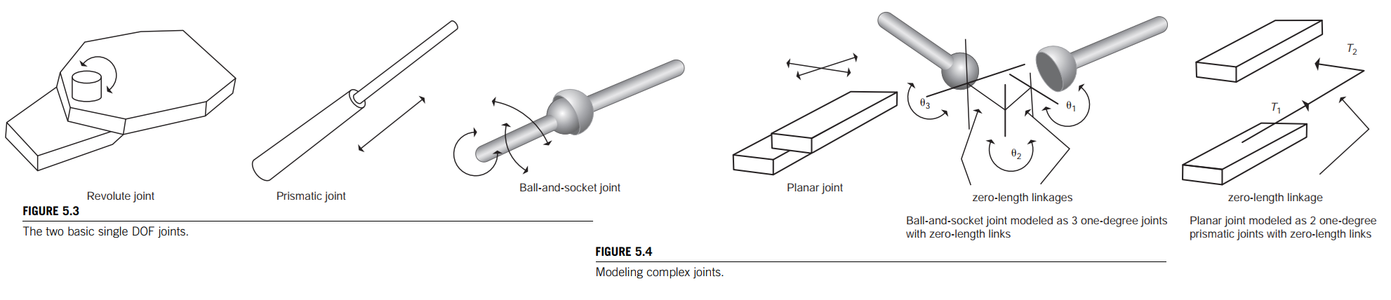
The joints of Figure 5.3 allow motion in one direction and are said to have one degree of freedom (DOF). Structures in which more than one DOF are coincident are called complex joints. Complex joints include the planar joint and the ball-and-socket joint.

Data structure for hierarchical modeling

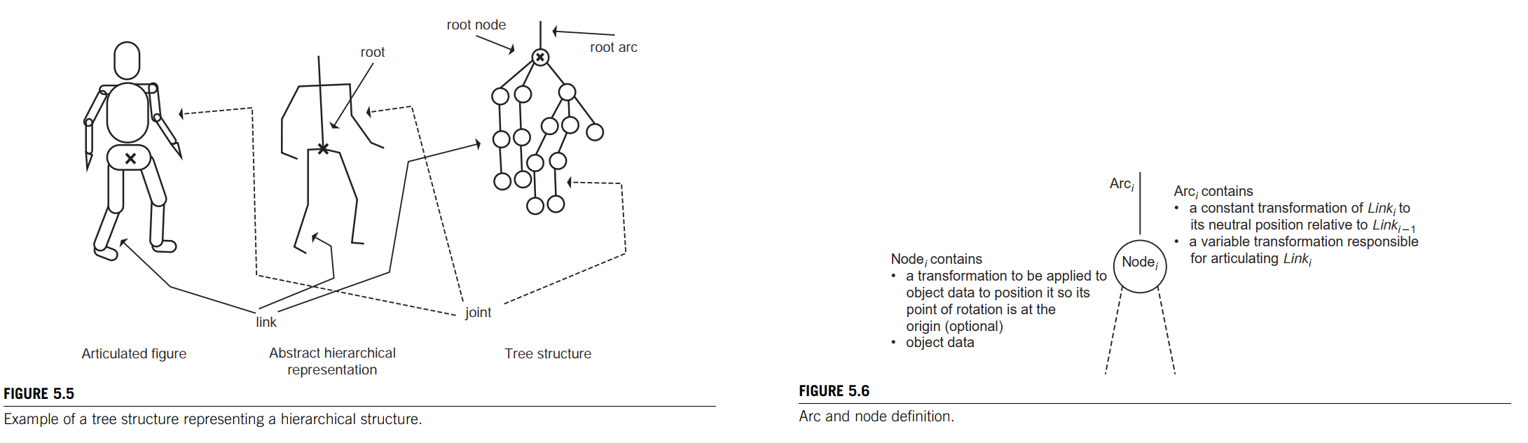
The mapping between the hierarchy and tree structure relates a node of the tree to information about the object part (the link) and relates an arc of the tree (the joint) to the transformation to apply to all of the nodes below it in the hierarchy.

树的结点对应是人体骨骼，树的边对应是转换矩阵（关节点做origin）, T-Pose或者A-Pose状态下就是顶点在子骨骼空间的坐标–>顶点在父骨骼空间坐标的转换矩阵，e.g.
$$
T_1 Link_1 = Link_0空间下的坐标
$$

Relating a tree arc to a figure joint may seem counterintuitive, but it is convenient because a node of the tree can have several arcs emanating from it, just as an object part may have several joints attached to it.

A simple example

👉Coordinate Systems in Algebra >>

In this example, there is assumed to be no transformation at any of the nodes; the data are defined in a position ready for articulation.（T-pose, A-pose）

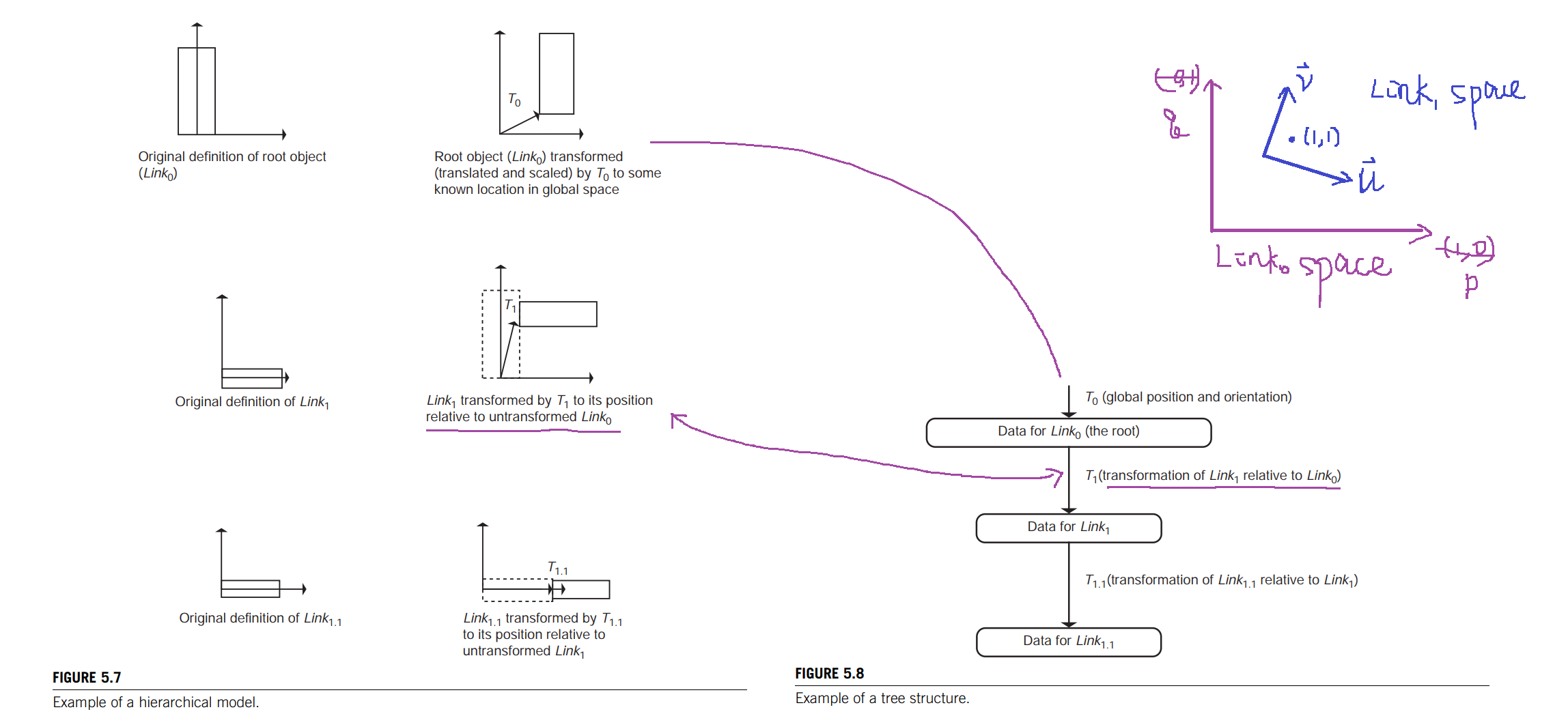
the data are defined in a position ready for articulation. $Link_0$, the root object, is transformed to its orientation and position in global space by $T_0$.
$$
T_0
\begin{bmatrix}
1 & 0 & 0\\ 0 & 1 & 0\\ 0 & 0 & 1
\end{bmatrix}是Link_0的坐标基矩阵
\begin{bmatrix}
p & q
\end{bmatrix}
$$
Because all of the other parts of the hierarchy will be defined relative to this part, this transformation affects the entire assemblage of parts and thus will transform the position and orientation of the entire structure. This transformation can be changed over time in order to animate the position and orientation of the rigid structure.

$Link_1$ is defined relative to the untransformed root object by transformation $T_1$.

Similarly, $Link_{1.1}$ is defined relative to the untransformed $Link_1$ by transformation $T_{1.1}$. These relationships can be represented in a tree structure by associating the links with nodes and the transformations with arcs.

In the example shown in Figure 5.8, the articulation transformations are not yet included in the model.

The vertices of a particular object can be transformed to their final positions by concatenating the transformations higher up the tree and applying the composite transformation matrix to the vertices.
注意，是顶点，是点坐标

A vertex, $V_0$, of the root object, $Link_0$, is located in the world coordinate system, $V_0’$ by applying the rigid transformation that affects the entire structure; see Equation 5.1. (顶点$V_0$在$Link_0$骨骼空间下的坐标转换成了在世界坐标系standard coordinate下的坐标$V_0’$)
$$
V_0’ = T_0 V_0
\tag{5.1}
$$
A vertex of the $Link_1$ object is located in the world coordinate system by transforming it first to its location relative to $Link_0$ and then relocating it (conceptually along with $Link_0$) to world space by Equation 5.2.
$$
V_1’ = T_0T_1V_1
\tag{5.2}
$$

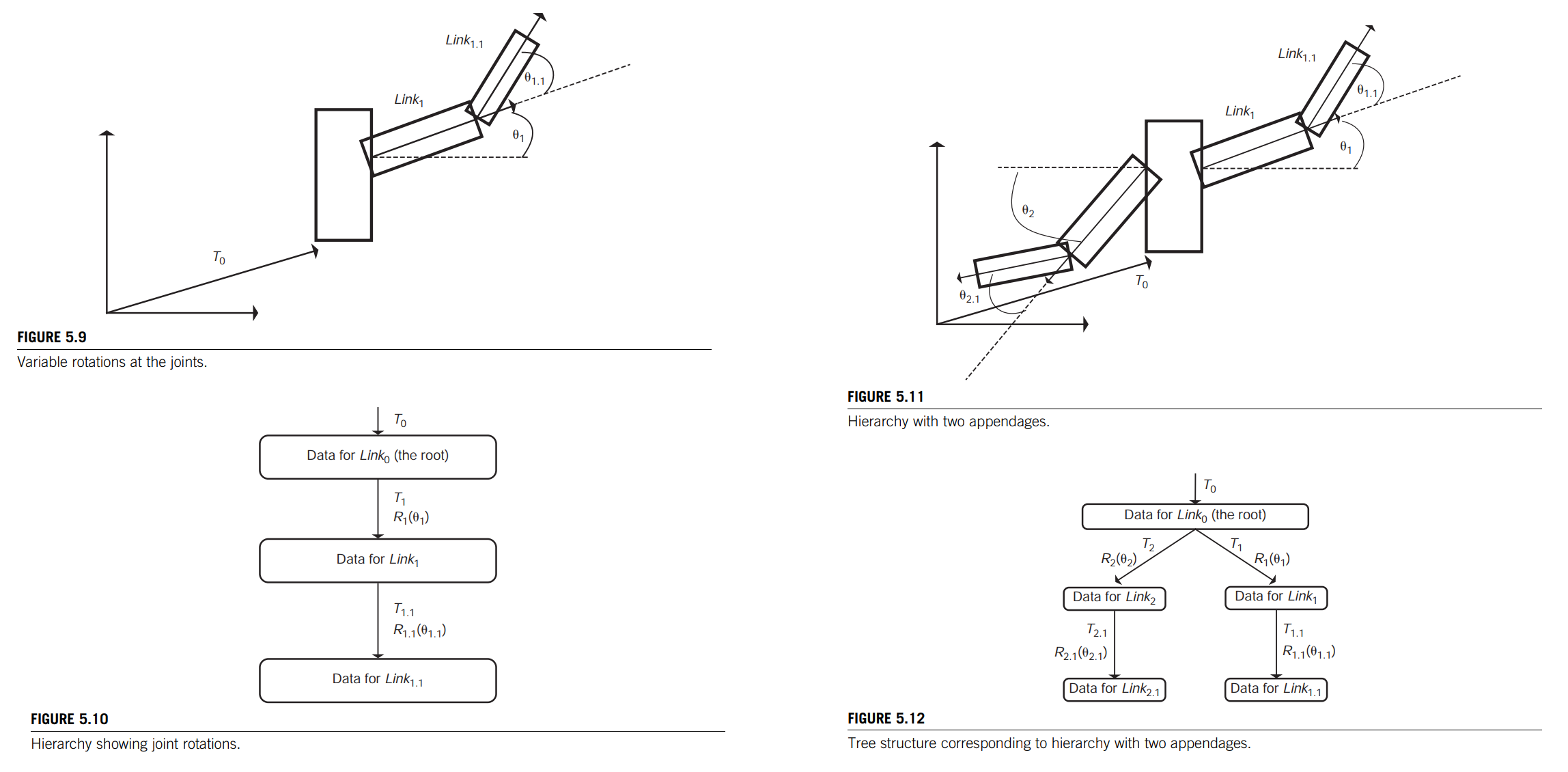
To locate a vertex of $Link_1$ in world space, one must first transform it via the joint rotation matrix(关节旋转矩阵). Once that is complete, then the rest of the transformations up the hierarchy are applied (see Eq. 5.4).(Figure5.9,5.10)
$$
V_1’ = T_0T_1R_1(\theta_1) V_1
\tag{5.4}
$$
A vertex of $Link_{1.1}$ is transformed similarly by compositing all of the transformations up the hierarchy
to the root, as in Equation 5.5.
$$
V_{1.1}’ = T_0T_1R_1(\theta_1) T_{1.1}R_{1.1}(\theta_{1.1})V_{1.1}
\tag{5.5}
$$
For example Figure5.11,5.12, in a simplified human figure, the root hip area (see Figure 5.5) might branch into the torso and two legs. If prismatic joints are used, the strategy is the same; the only difference is that the rotation transformation of the joint (arc) is replaced by a translation.

Local coordinate frames

In setting up complex hierarchies and in applying computationally involved procedures such as IK, it is convenient to be able to define points in the local coordinate system (frame) associated with a joint and to have a well-defined method for converting the coordinates of a point from one frame to another. A common use for this method is to convert points defined in the frame of a joint to the global coordinate system for display purposes.

Forward kinematics

Traversal follows a depth-first pattern 深搜 from root to leaf node. The traversal then backtracks up回溯 the tree until an unexplored downward arc is encountered.

The downward arc is then traversed, followed by backtracking up to find the next unexplored arc.

This traversal continues until all nodes and arcs have been visited.

Whenever an arc is followed down the tree hierarchy, its transformations are concatenated to the transformations of its parent node.
Whenever an arc is traversed back up the tree to a node, the transformation of that node must be restored before traversal continues downward.

each arc has associated with it the following:

• nodePtr: A pointer to a node that holds the data to be articulated by the arc.
• Lmatrix: A matrix that locates the following (child) node relative to the previous (parent) node. 骨骼空间转换矩阵
• Amatrix: A matrix that articulates the node data; this is the matrix that is changed in order to animat (articulate) the linkage. 骨骼运动矩阵
• arcPtr: A pointer to a sibling arc (another child of this arc’s parent node); this is NULL if there are no more siblings.

Each node has associated with it the following:

• dataPtr: Data (possibly shared by other nodes) that represent the geometry of this segment of the figure.
• Tmatrix: A matrix to transform the node data into position to be articulated (e.g., put the point of rotation at the origin).
• ArcPtr: A pointer to a single child arc.

1
2
3
4
5
6
7
8
9
10
11
12
13
14
15
16
17
18
19
20
21
22
23
24
25
26
27
28
29
30
31

traverse(arcPtr,matrix)
{
    //get transformations of arc and concatenate to current matrix
    matrix = matrix * arcPtr->Lmatrix // concatenate location
    matrix = matrix * arcPtr->Amatrix // concatenate articulation
    // process data at node
    nodePtr = arcPtr->nodePtr // get the node of the arc
    push(matrix) // save the matrix
    matrix = matrix * nodePtr->matrix // ready for articulation

    articulatedData = transformData(matrix,dataPtr) // articulate the data
    draw(articulatedData)// // and draw it

    matrix = pop() // restore matrix for node’s children

    // process children of node
    if (nodePtr->arcPtr!= NULL) 
    { 
        // if not a terminal node
        nextArcPtr = nodePtr->arcPtr // get first arc emanating from node
        while (nextArcPtr != NULL) 
        { 
            // while there’s an arc to process
            push(matrix) // save matrix at node
            traverse(nextArcPtr,matrix) // traverse arc
            matrix = pop() // restore matrix at node
            nextArcPtr = nextArcPtr->arcPtr // set next child of node
        }
    }
}
traverse(rootArcPtr,I) // ‘I’ is identity matrix

In a simple animation, a user may determine a key position interactively or by specifying numeric values and then interpolate the joint values between key positions.

Specifying all of the joint parameter values for key positions is called forward kinematics and is an easy way to animate the figure.

A completely specified set of linkage parameters, which results in positioning the hierarchical figure, are called a pose. A pose is specified by a vector (the pose vector) consisting of one parameter for each DOF.

Inverse kinematics

In IK, the desired position and possibly orientation of the end effector are given by the user along with the initial pose vector. From this, the joint values required to attain that configuration are calculated, giving the final pose vector.

If there are so many constraints on the configuration that no solution exists, the system is called overconstrained.

If there are relatively few constraints on the system and there are many solutions to the problem posed, then it is underconstrained.

The reachable workspace is that volume which the end effector can reach.

The dexterous workspace is the volume that the end effector can reach in any orientation.

Solving a simple system by analysis

Assume for now (without loss of generality) that the base is at the origin. In a simple IK problem, the user gives the $(X, Y)$ coordinate of the desired position for the end effector.

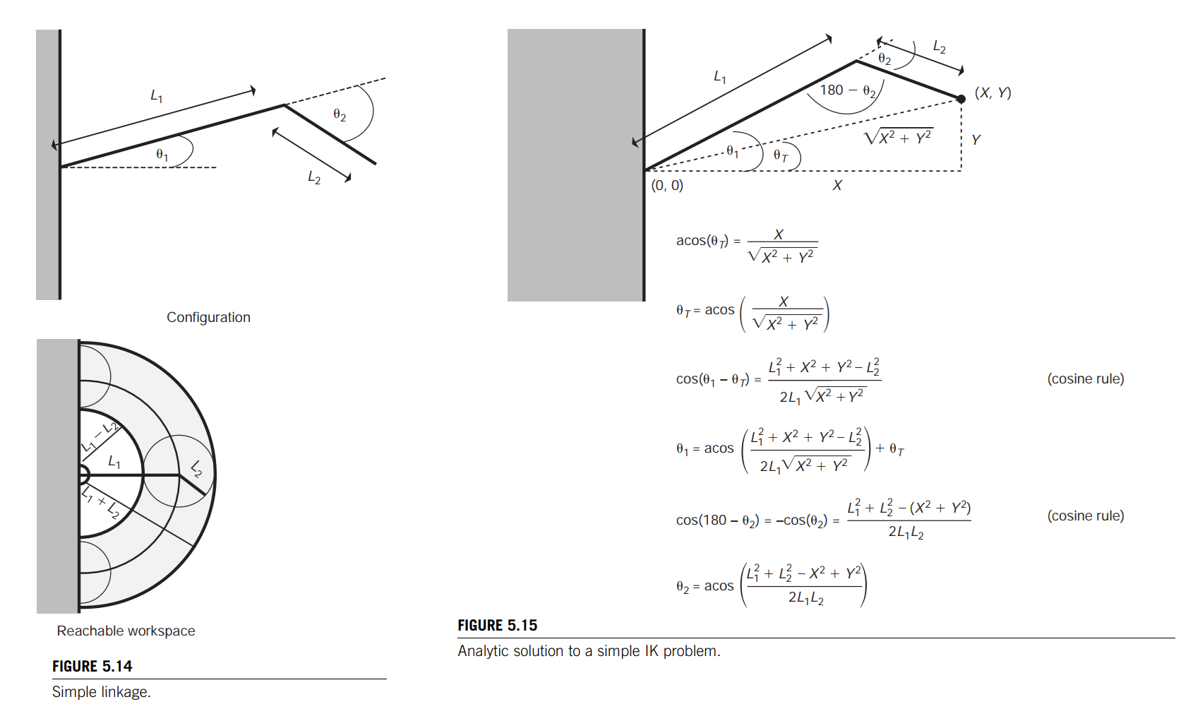
The joint angles, $\theta_1$ and $\theta_2$, can be determined by computing the distance from the base to the goal and using the law of cosines to compute the interior angles.

Most linkages used in robotic applications are designed to be simple enough for this algebraic manipulation. However, for many cases that arise in computer animation, analytic solutions are not tractable. In such cases, iterative numeric solutions must be relied on.

The Jacobian

At each time step, a computation is performed that determines a way to change each joint angle in order to direct the current position and orientation of the end effector toward the desired configuration. There are several methods used to compute the change in joint angle, but most involve forming the matrix of partial derivatives called the Jacobian.

👉Partial Calculus >>

Given specific values for the input variables, $x_i$, each of the output variables, $y_i$, can be computed by its respective function.
$$
y_1 = f_1(x_1, x_2, x_3, \cdots, x_6)\\
\cdots \\
y_6 = f_6(x_1, x_2, x_3, \cdots, x_6)
\tag{5.6}
$$
The differentials of $y_i$ can be written in terms of the differentials of $x_i$ using the chain rule. This generates Equation 5.7.
$$
dy_i = \frac{\partial f_i}{\partial x_1} dx_1 + \cdots + \frac{\partial f_i}{\partial x_6} dx_6
\tag{5.7}
$$

Equations 5.6 and 5.7 can be put in vector notation, producing Equations 5.8 and 5.9, respectively.
$$
d\pmb{Y} = \frac{\partial \pmb{F}}{\partial \pmb{X}} d \pmb{X}
\tag{5.8}
$$
A matrix of partial derivatives, $\frac{\partial \pmb{F}}{\partial \pmb{X}}$, is called the Jacobian and is a function of the current values of $x_i$.

The Jacobian can be thought of as mapping the velocities of $\pmb{X}$ to the velocities of $\pmb{Y}$ (Eq. 5.10).
$$
\dot{\pmb{Y}} = \pmb{J(X)}\dot{\pmb{X}}
\tag{5.10}
$$

When one applies the Jacobian to a linked appendage, the input variables, $x_i$, become the joint values and the output variables, $y_i$, become the end effector position and orientation (in some suitable representation such as $x-y-z$ fixed angles).
$$
\pmb{Y} = \begin{bmatrix}
p_x & p_y & p_z & \alpha_x & \alpha_y & \alpha_z
\end{bmatrix}^T
\tag{5.11}
$$
In this case, the Jacobian relates the velocities of the joint angles, $\dot{\theta}$, to the velocities of the end effector position and orientation, $\pmb{\dot{Y}}$ (Eq. 5.12).
$$
\pmb{V} = \pmb{\dot{Y}} = \pmb{J}(\theta) \dot{\theta}
\tag{5.12}
$$
where, $\pmb{V}$ is the vector of linear and rotational velocities and represents the desired change in the end effector.
$$
\pmb{V} = \begin{bmatrix}
v_x & v_y & v_z & \omega_x & \omega_y & \omega_z
\end{bmatrix}^T
\tag{5.13}
$$
$\pmb{J}$, the Jacobian, is a matrix that relates the two and is a function of the current pose
$$
\pmb{J} = \begin{bmatrix}
\frac{\partial p_x}{\partial \theta_1} & \frac{\partial p_x}{\partial \theta_2} & \cdots& \frac{\partial p_x}{\partial \theta_n}\\
\frac{\partial p_y}{\partial \theta_1} & \frac{\partial p_y}{\partial \theta_2} & \cdots & \frac{\partial p_y}{\partial \theta_n}\\
\cdots & \cdots & \cdots & \cdots\\
\frac{\partial \alpha_z}{\partial \theta_1} & \frac{\partial \alpha_z}{\partial \theta_2} & \cdots & \frac{\partial \alpha_z}{\partial \theta_n}
\end{bmatrix}
\tag{5.15}
$$

Each term of the Jacobian relates the change of a specific joint to a specific change in the end effector.

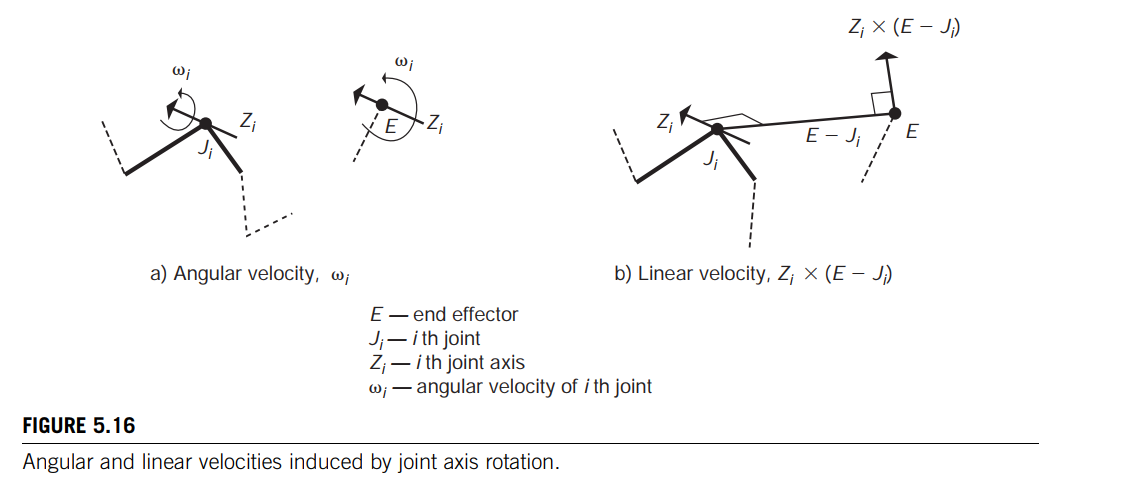
For a revolute joint, the rotational change in the end effector, $\omega$, is merely the velocity of the joint angle about the axis of revolution at the joint under consideration. 对于一个转动关节， 末端执行器的旋转变化，$\omega$，仅仅是关节角绕转轴的速度。

For a prismatic joint, the end effector orientation is unaffected by the joint articulation. 对于移动关节，末端执行器方向不受关节运动的影响。

For a rotational joint, the linear change in the end effector is the cross-product of the axis of revolution and a vector from the joint to the end effector. The rotation at a rotational joint induces an instantaneous linear direction of travel at the end effector. 对于一个旋转关节，末端执行器的线性变化是旋转轴和一个从关节到末端执行器的向量的叉积。旋转关节上的旋转会在末端执行器上产生瞬时的线性运动方向。
For a prismatic joint, the linear change is identical to the change at the joint (see Figure 5.16). 对于移动关节，线性变化等于关节处的变化。

In forming the Jacobian matrix, this information must be converted into some common coordinate system such as the global inertial (world) coordinate system or the end effector coordinate system.

A simple example

In this example, the objective is to move the end effector, $E$, to the goal position, $G$. The orientation of the end effector is of no concern in this example.

The axis of rotation of each joint is perpendicular to the figure, coming out of the paper. 关节的旋转轴朝向读者

The effect of an incremental rotation, $g_i$, of each joint can be determined by the cross-product of the joint axis and the vector from the joint to the end effector, $V_i$ (Figure 5.18), and form the columns of the Jacobian.

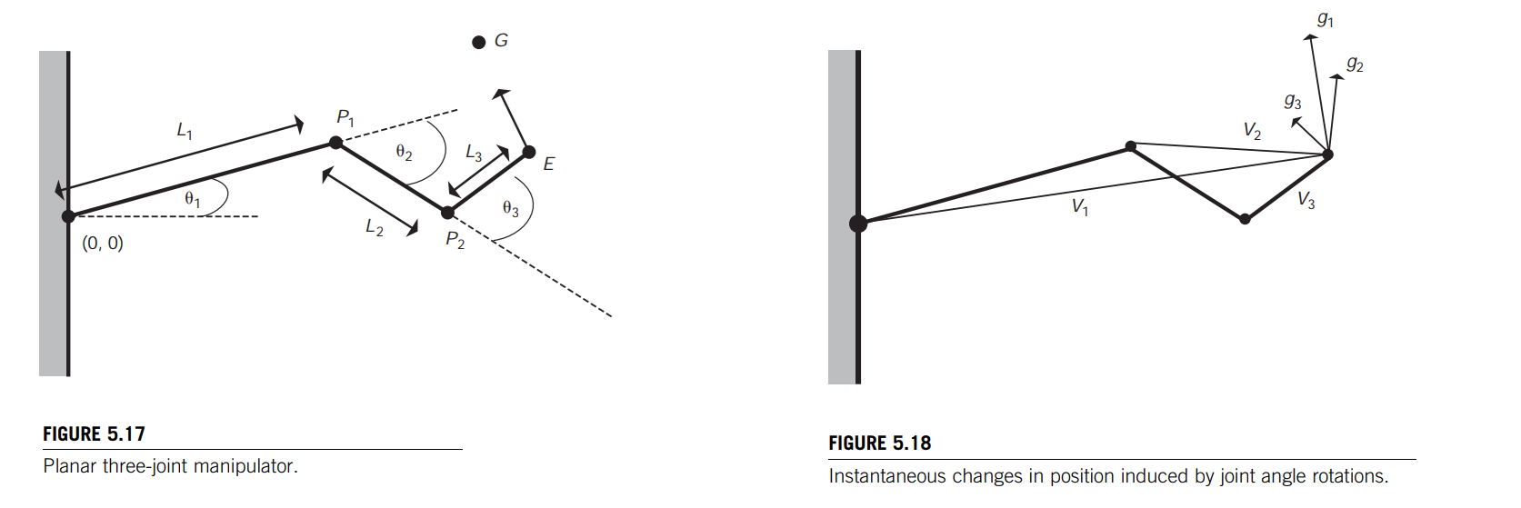
A vector of the desired change in values is set equal to the Jacobian matrix (Eq. 5.17) multiplied by a vector of the unknown values, which are the changes to the joint angles.

where desired change is,
$$
V = \begin{bmatrix}
(G-E)_x\\
(G-E)_y\\
(G-E)_z
\end{bmatrix}
$$
Jacobian matrix is,
$$
J =
\begin{bmatrix}
((0,0,1) \times E)_x & ((0,0,1) \times (E - P_1))_x & ((0,0,1) \times (E - P_2))_x\\
((0,0,1) \times E)_y & ((0,0,1) \times (E - P_1))_y & ((0,0,1) \times (E - P_2))_y\\
((0,0,1) \times E)_z & ((0,0,1) \times (E - P_1))_z & ((0,0,1) \times (E - P_2))_z
\end{bmatrix}
\tag{1.57}
$$

从几何意义上来求Jacobian矩阵，就是这种叉乘的做法

Numeric solutions to IK

Solution using the inverse Jacobian

If the inverse of the Jacobian ($J^{-1}$) does not exist, then the system is said to be singular for the given joint angles. (奇异 = 不可逆)

A singularity occurs when a linear combination of the joint angle velocities cannot be formed to produce the desired end effector velocities. 大部分情况下，$J^{-1}$都是直接求不出来的

$$
V = J\dot{\theta}
\tag{5.18}
$$

$$
J^{-1}V = \dot{\theta}
\tag{5.19}
$$

👉Inverse Matrix in Algebra >>

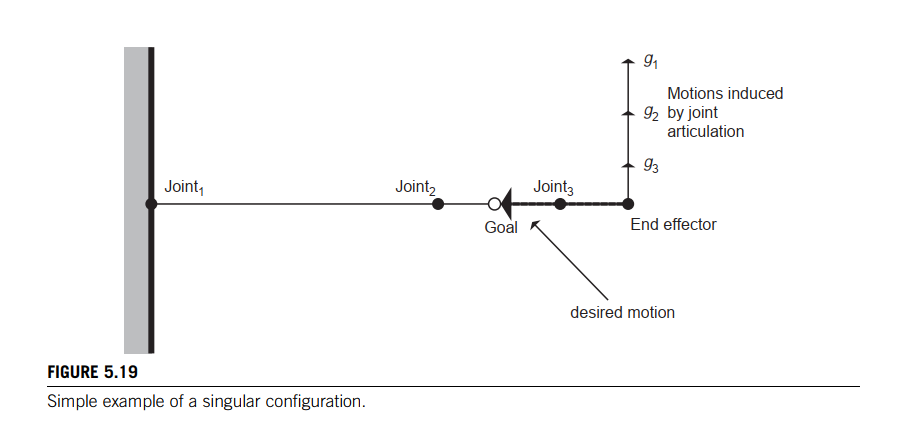
As shown in Figure5.19, a change in each joint angle would produce a vector perpendicular to the desired direction. Obviously, no linear combination of these vectors could produce the desired motion vector.

Problems with singularities can be reduced if the manipulator is redundant—when there are more DOF than there are constraints to be satisfied. In this case, the Jacobian is not a square matrix and, potentially, there are an infinite number of solutions to the IK problem. 自由度大于约束的时候，可以减少奇点问题, 再这种情况下，Jacobian矩阵不是方阵，对于IK问题可能会存在很多个解

If the columns of $J$ are linearly independent(i.e., $J$ has full column rank, 此时$J$是一个高瘦矩阵，比如$9 \times 3$), the $(J^TJ)^{-1}$ exists and instead, the pseudoinverse, $J^{\dagger}$ an be used as in Equation 5.20.

$$
V = J\dot{\theta}\\
J^TV = J^TJ\dot{\theta}\\
(J^TJ)^{-1}J^TV = \dot{\theta}\\
J^{\dagger}V = \dot{\theta}
\tag{5.20}
$$

understand pseudoinverse from least squares view:

The pseudoinverse maps the desired velocities of the end effector to the required changes of the joint angles.

If the rows of $J$ are linearly independent, 此时$J$是一个矮胖矩阵，比如$3 \times 9$。
$$
J^{\dagger} = J^T(JJ^T)^{-1}
$$
👉LU decomposition >> can be used to solve Equation.
$$
J^{\dagger}V = \dot{\theta}\\
J^T(JJ^T)^{-1}V = \dot{\theta}\\
$$
first, get $\beta$ value,
$$
\beta = (JJ^T)^{-1}V
\tag{5.22}
$$
then get $\dot{\theta}$ value
$$
(JJ^T)\beta = V\\
J^T\beta = \dot{\theta}
\tag{5.23}
$$

Simple 👉Euler integration can be used at this point to update the joint angles. The Jacobian has changed at the next time step, so the computation must be performed again and another step taken. This process repeats until the end effector reaches the goal configuration within some acceptable (i.e., user-defined) tolerance.

通常会用👉Gaussian-Newton法对应Jacobian pseudoinverse方法

For example:

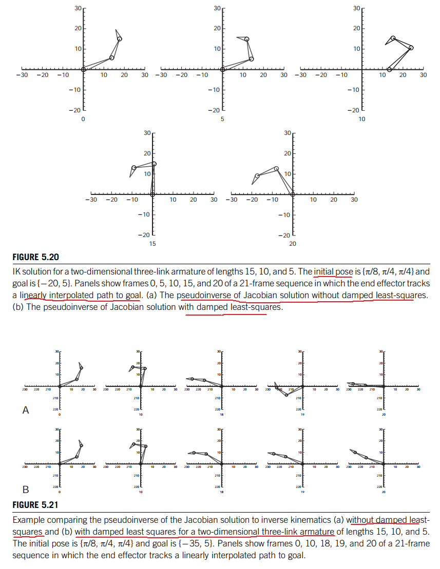
Even the underconstrained case still has problems with singularities，也就是说即便使用伪逆的方法来求解，有时候计算机精度的问题，可能还是不可逆，解决这个问题可以加上damp. A proposed solution to such bad behavior is the damped least-squares approach [1] [2]. Referring to Equation 5.24, a user-supplied parameter is used to add in a term that reduces the sensitivity of the pseudoinverse.
$$
\dot{\theta} = J^T(JJ^T + \lambda^2I)^{-1}V
\tag{5.24}
$$

Adding more control

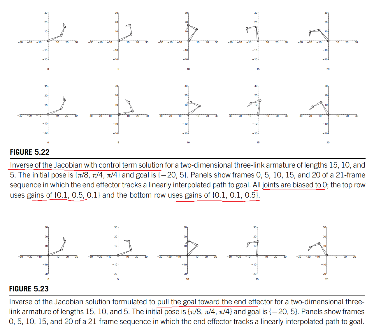
To better control the kinematic model such as encouraging joint angle constraints, a control expression can be added to the pseudoinverse Jacobian solution.The form for the control expression is shown in Equation 5.25.

$$
\dot{\theta} = (J^{\dagger}J - I)z
\tag{5.25}
$$
In Equation 5.26 it is shown that a change to pose parameters in the form of Equation 5.25 does not add anything to the velocities.

$$
V = J\dot{\theta}\\
V = J(J^{\dagger}J - I)z\\
V = (JJ^{\dagger}J - J)z\\
V = 0z\\
V = 0
\tag{5.26}
$$

To bias the solution toward specific joint angles, such as the middle angle between joint limits, $z$ is defined as in Equation 5.27(因为关节角的转动给了一定的约束，所以要尽量的使solution偏向约束下的关节角度)
$$
z = \alpha_i(\theta_i - \theta_{ci})^2
\tag{5.27}
$$
where, $\theta_i$ are the current joint angles, $\theta_{ci}$ are the desired joint angles, and $\alpha_i$ are the joint gains.

The desired angles and gains are input parameters. The gain indicates the relative importance of the associated desired angle; the higher the gain, the stiffer the joint 增益越高，关节越硬.If the gain for a particular joint is high, then the solution will be such that the joint angle quickly approaches the desired joint angle.

The control expression is added to the conventional pseudoinverse of the Jacobian (Eq. 5.28).
$$
\dot{\theta} = J^{\dagger}V + (J^{\dagger}J - I)z
\tag{5.28}
$$

Alternative Jacobian

Instead of trying to push the end effector toward the goal position, a formulation has been proposed that pulls the goal to the end effector [1].

Avoiding the inverse: using the transpose of the Jacobian

the vector of joint parameter changes is formed by multiplying the transpose of the Jacobian times the velocity vector and using a scaled version of this as the joint parameter change vector.
$$
\dot{\theta} = \alpha J^TV
$$

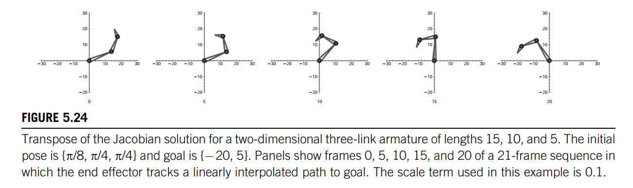
这也是求解优化问题的梯度下降法

Procedurally determining the angles: cyclic coordinate descent CCD

Cyclic coordinate descent considers each joint one at a time, sequentially from the outermost inward [5]. At each joint, an angle is chosen that best gets the end effector to the goal position.

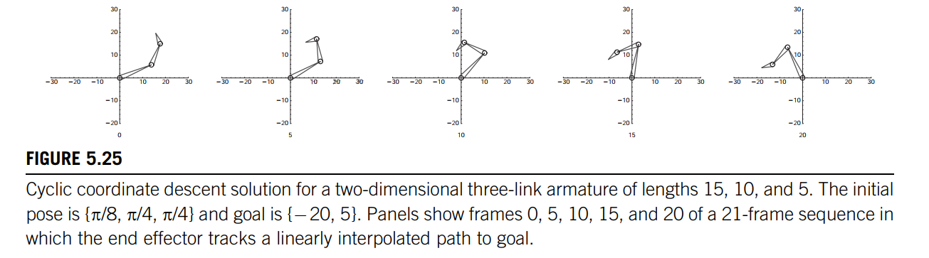
CCD很简单，就是对于每个关节点都让这个关节点旋转一定角度，从而使end effector离目标点最近

[5] Welman C. Inverse Kinematics and Geometric Constraints for Articulated Figure Manipulation. M.S. Thesis. Simon Frasier University; 1993.

Chapter summary

numeric approach is often needed. Trade-offs among the numeric approaches include ease of implementation, possible real-time behavior, and robustness in the face of singularities.

An additional approach is targeted at linkages that are specifically human-like in their DOF and heuristically solves reaching problems by trying to model human-like reaching; this is discussed in Chapter 9.

IK Survey:
http://www.andreasaristidou.com/publications/papers/IK_survey.pdf