NumericalAnalysis-C2-Systems-of-Equations

Keywords: Gaussian Elimination, LU Factorization, Jacobi Matrix, Jacobi Iterative Method, Symmetric positve-definite matrice, Nonlinear Systems, Mathlab

This is the Chapter2 ReadingNotes from book Numerical Analysis by Timothy.

Gaussian Elimination

Consider the system
$$
\begin{cases}
x + y = 3\\
3x - 4y = 2
\end{cases}
\tag{2.1}
$$

Naive Gaussian Elimination

The advantage of the tableau form is that the variables are hidden during elimination.（其实就是增广矩阵, 矩阵行变换，最简阶梯式求解的过程就叫消元）
$$
\begin{bmatrix}
1 & 1 & 3\\
3 & -4 & 1
\end{bmatrix}
\longrightarrow
\begin{bmatrix}
1 & 1 & 3\\
0 & -7 & -7
\end{bmatrix}
$$
the corresponding equation is:
$$
\begin{cases}
x + y = 3\\
-7y = -7
\end{cases}
$$
we solve y, x in order, this part is called back substitution, or backsolving.

Operation counts

The general form of the tableau for $n$ equations in $n$ unknowns is
$$
\begin{bmatrix}
a_{11} & a_{12} & \cdots & a_{1n} & | & b_1\\
a_{21} & a_{22} & \cdots & a_{2n} & | & b_2\\
\cdots & \cdots & \cdots & \cdots & | & \cdots\\
a_{n1} & a_{n2} & \cdots & a_{nn} & | & b_n\\
\end{bmatrix}
$$

The elimination process can be written as:

1
2
3
4
5

for j = 1 : n-1
    for i = j+1 : n
        eliminate entry a(i,j)
    end
end

This number and the other numbers $a_{ii}$ that are eventually divisors（除数） in Gaussian elimination are called pivots.

More specific of elimination process:

1
2
3
4
5
6
7
8
9
10
11
12
13
14

//column
for j = 1 : n-1
    if abs(a(j,j))<eps; error(’zero pivot encountered’); end
    //row
    for i = j+1 : n
        mult = a(i,j)/a(j,j);
        //elements in this row
        for k = j+1:n
            a(i,k) = a(i,k) - mult * a(j,k);
        end
        //diagnal element
        b(i) = b(i) - mult*b(j);
    end
end

For the operation, we can see that:

$$
\begin{bmatrix}
a_{11} & a_{12} & \cdots & a_{1n} & | & b_1\\
a_{21} & a_{22} & \cdots & a_{2n} & | & b_2\\
\end{bmatrix}
\longrightarrow
\begin{bmatrix}
a_{11} & a_{12} & \cdots & a_{1n} & | & b_1\\
0 & a_{22} - \frac{a_{21}}{a_{11}}a_{12} & \cdots & a_{2n} - \frac{a_{21}}{a_{11}}a_{1n} & | & b_2 - \frac{a_{21}}{a_{11}}b_1\\
\end{bmatrix}
$$
Accounting for the operations, this requires one division (to find the multiplier $\frac{a_{21}}{a_{11}}$), plus $n$ multiplications and $n$ additions, which is $2n+1$.

The total operations in the matrix is
$$
\begin{bmatrix}
0\\
2n+1 & 0\\
2n+1 & 2(n-1)+1 & 0\\
2n+1 & 2(n-1)+1 & 2(n-2)+1\\
\cdots & \cdots & \cdots \\
2n+1 & 2(n-1)+1 & 2(n-2)+1 & \cdots & 2(3)+1 & 0\\
2n+1 & 2(n-1)+1 & 2(n-2)+1 & \cdots & 2(3)+1 & 2(2) + 1 & 0\\
\end{bmatrix}
$$
We total up the operation as
$$
\begin{aligned}
\sum_{j=1}^{n-1}\sum_{i=1}^{j} 2(j+1) + 1 &= \frac{2}{3}n^3 + \frac{1}{2}n^2 -\frac{7}{6}n
\end{aligned}
$$
The operation count shows that direct solution of $n$ equations in $n$ unknowns by Gaussian elimination is an $O(n^3)$ process.

The back-substitution step is:

1
2
3
4
5
6

for i = n : -1 : 1
    for j = i+1 : n
        b(i) = b(i) - a(i,j)*x(j);
    end
    x(i) = b(i)/a(i,i);
end

Counting operations yield
$$
1 + 3 + 5 + \cdots + (2n-1) = n^2
$$

The computer can carry out $(5000)^2$ operations in $0.1$ seconds, or $(5000)^2(10) =
2.5 × 10^8$ operations/second.

The $LU$ Factorization

Matrix form of Gaussian elimination

DEFINITION 2.2
An $m \times n$ matrix $L$ is lower triangular if its entries satisfy $l_{ij} = 0$ for $i < j$. An $m \times n$ matrix $U$ is upper triangular if its entries satisfy $u_{ij} = 0$ for $i > j$.

💡For example💡:

Fine the $LU$ factorization of
$$
A = \begin{bmatrix}
1 & 2 & -1\\
2 & 1 & -2\\
-3 & 1 & 1
\end{bmatrix}
\tag{2.13}
$$

Solution:

$$
A = \begin{bmatrix}
1 & 2 & -1\\
2 & 1 & -2\\
-3 & 1 & 1
\end{bmatrix}
\xrightarrow[from \space row \space 2]{substract \space 2 \times row \space 1 }
\begin{bmatrix}
1 & 2 & -1\\
0 & -3 & 0\\
-3 & 1 & 1
\end{bmatrix}
\xrightarrow[from \space row \space 3]{substract \space 3 \times row \space 1 }
\begin{bmatrix}
1 & 2 & -1\\
0 & -3 & 0\\
0 & 7 & -2
\end{bmatrix}
\xrightarrow[from \space row \space 3]{substract \space -\frac{7}{3} \times row \space 2 }
\begin{bmatrix}
1 & 2 & -1\\
0 & -3 & 0\\
0 & 0 & -2
\end{bmatrix} = U
$$

The lower triangular $L$ matrix is formed, as in the previous example, by putting $1$’s on the main diagonal and the multipliers in the lower triangle—in the specific places they were used for elimination. That is,
$$
L =
\begin{bmatrix}
1 & 0 & 0\\
2 & 1 & 0\\
-3 & -\frac{7}{3} & 1
\end{bmatrix}
\tag{2.14}
$$

Back substitution with the LU factorization

$Ax = b$
(a) Solve $Lc = b$ for $c$.
(b) Solve $Ux = c$ for $x$.

Complexity of the LU factorization

Now, suppose that we need to solve a number of different problems with the same $A$ and different $b$. That is, we are presented with the set of problems
$$
Ax = b_1, \\
Ax = b_2, \\
…\\
Ax = b_k\\
$$
with naive Gaussian Elimination, the complexity is
$$
\frac{2kn^3}{2} + kn^2
$$

but with $LU$, the complesity is

$$
\underbrace{\frac{2n^3}{3}}_{LU \space Factorization} + \underbrace{2kn^2}_{back \space substitutions}
$$

The $LU$ approach allows efficient handling of all present and future problems that involve the same coefficient matrix $A$.

Source of Error

Error magnification and condition number

DEFINITION 2.3
The infinity norm, or maximum norm, of the vector $x = (x_1, \cdots , x_n)$ is $||x||_\infty = max|x_i|$, $i = 1,\cdots,n$, that is, the maximum of the absolute values of the components of $x$.

DEFINITION 2.4
Let $x_a$ be an approximate solution of the linear system $Ax = b$. The residual is the vector $r = b − Ax_a$. The backward error is the norm of the residual $||b − Ax_a||_\infty$, and the forward error is $||x − x_a||_\infty$.

💡For example💡:

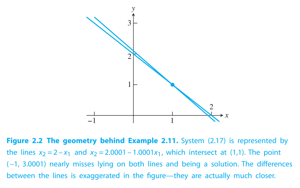
Find the forward and backward errors for the approximate solution $[−1,3.0001]$ of the system
$$
\begin{cases}
x_1 + x_2 = 2\\
1.0001x_1 + x_2 = 2.0001.
\end{cases}
\tag{2.17}
$$

Solution:

The correct solution is
$$
[x_1, x_2] = [1,1]
$$

The backward error is the infinity norm of the vector
$$
b - Ax_a =
\begin{bmatrix}
-0.0001\\
0.0001
\end{bmatrix}
$$
which is $0.0001$.

The forward error is the infinity norm of the difference

$$
x - x_a =
\begin{bmatrix}
2\\
−2.0001
\end{bmatrix}
$$
which is $2.0001$.

Figure 2.2 helps to clarify how there can be a small backward error and large forward error at the same time. Even though the “approximate root’’ $(−1,3.0001)$ is relatively far from the exact root $(1,1)$, it nearly lies on both lines. This is possible because the two lines are almost parallel. If the lines are far from parallel, the forward and backward errors will be closer in magnitude.

Denote the residual by $r = b - Ax_a$. The relative backward error of system $Ax = b$
is defined to be
$$
\frac{||r||_\infty}{||b||_\infty}
$$

and the relative forward error is

$$
\frac{||x - x_a||_\infty}{||x||_\infty}
$$

The error magnification factor for $Ax = b$ is the ratio of the two, or
$$
error-magnification-factor = \frac{relative-forward-error}{relative-backward-error} = \frac{\frac{||x - x_a||_\infty}{||x||_\infty}}{\frac{||r||_\infty}{||b||_\infty}}
\tag{2.18}
$$

For system(2.17), the error magnification factor is
$$
\frac{\frac{2.0001}{1}}{\frac{0.0001}{2.0001}} \approx 40004.0001
$$

DEFINITION 2.5
The condition number of a square matrix $A$, $cond(A)$, is the maximum possible error magnification factor for solving $Ax = b$, over all right-hand sides $b$.
Surprisingly, there is a compact formula for the condition number of a square matrix. Analogous to the norm of a vector, define the matrix norm of an $n \times n$ matrix $A$ as
$$
||A||_\infty = maximum-absolute-row-sum
\tag{2.19}
$$

THEOREM 2.6
The condition number of the $n \times n$ matrix $A$ is
$$
cond(A) = ||A|| \cdot ||A^{-1}||
$$

Thus, The norm of
$$
A =
\begin{bmatrix}
1 & 1\\
1.0001 & 1
\end{bmatrix}
$$
is $||A|| = 2.0001$

The condition number of $A$ is

$$
cond(A) = 40004.0001.
$$

This is exactly the error magnification we found in Example above, which evidently achieves the worst case, defining the condition number. The error magnification factor for any other $b$ in this system will be less than or equal to $40004.0001$.

If $cond(A) ≈ 10^k$, we should prepare to lose $k$ digits of accuracy in computing $x$.

In the example above, since $cond(A) \approx 40004.0001$. so in double precision we should expect about $16 − 4 = 12$ correct digits in the solution $x$.

We use Matlab for a computation:

1
2
3
4
5

>> A = [1 1;1.0001 1]; b=[2;2.0001];
>> xa = A\b
xa =
1.00000000000222
0.99999999999778

Compared with the correct solution $x = [1,1]$, the computed solution has about $11$ correct digits, close to the prediction from the condition number.

vector norm $||x||$, which satisfies three properties:
(i) $||x|| \neq 0$ with equality if and only if $x = [0, . . . ,0]$
(ii) for each scalar $\alpha$ and vector $x$, $||\alpha x|| = |\alpha| \cdot ||x||$
(iii) for vectors $x,y$, $||x + y|| \leq ||x|| + ||y||$.

matrix norm $||A||\infty$ which satisfies three properties:
(i) $||A|| \geq 0$ with equality if and only if $A = 0$
(ii) for each scalar $\alpha$ and matrix $A$, $||\alpha A|| = |\alpha| \cdot ||A||$
(iii) for matrices $A,B$, $||A + B|| \leq ||A|| + ||B||$.

the vector 1-norm of the vector $x$ is $||x||_1 = |x_1| + |x_2| + \cdots + |x_n|$.

The matrix 1-norm of the $n \times n$ matrix $A$ is $||A||_1 = maximum-absolute
-column-sum$, which is the maximum of the 1-norms of the column vectors.

Swamping

💡For example💡:

$$
\begin{cases}
10^{-20}x_1 + x_2 = 1\\
x_1 + 2x_2 = 4
\end{cases}
$$
We will solve the system three times: once with complete accuracy, second where we mimic a computer following IEEE double precision arithmetic, and once more where we exchange the order of the equations first.

Solution:

1. Exact solution.

$$
\begin{bmatrix}
10^{-20} & 1 & | & 1\\
1 & 2 & | & 4
\end{bmatrix}
\xrightarrow[from \space row \space 2]{substract \space 10^{20} \times row \space 1 }
\begin{bmatrix}
10^{-20} & 1 & | & 1\\
0 & 2 - 10^{20} & | & 4 - 10^{20}
\end{bmatrix}
$$
The bottom equation is
$$
(2 - 10^{20}) x_2 = 4 - 10^{20}
\longrightarrow
x_2 = \frac{4 - 10^{20}}{2 - 10^{20}}
$$
and the top equation yields
$$
x_1 = \frac{-2 \times 10^{20}}{2 - 10^{20}}
$$
The exact solution is
$$
[x_1, x_2] \approx [2,1]
$$

2. IEEE double precision.

$2 - 10^{20}$ is the same as $-10^{20}$, due to rounding. $4 - 10^{20}$ is stored as $-10^{20}$

Thus,
$$
[x_1, x_2] = [0,1]
$$

3. IEEE double precision, after row exchange.
   $$
   \begin{bmatrix}
   1 & 2 & | & 4 \\
   10^{-20} & 1 & | & 1
   \end{bmatrix}
   \xrightarrow[from \space row \space 2]{substract \space 10^{-20} \times row \space 1 }
   \begin{bmatrix}
   1 & 2 & | & 4\\
   0 & 1 - 2 \times 10^{-20} & | & 1 - 4 \times 10^{-20}\\
   \end{bmatrix}
   $$

$1 - 2 \times 10^{-20}$ is stored as $1$, $1 - 4 \times 10^{-20}$ is stored as $1$.

$$
[x_1, x_2] = [2,1]
$$

The effect of subtracting $10^20$ times the top equation from the bottom equation was to overpower, or “swamp”, the bottom equation.

The $PA = LU$ Factorization

Partial pivoting

The partial pivoting protocol consists of comparing numbers before carrying out each elimination step.

(一种交换矩阵行的方法，用于避免因主对角线元素过小而导致的数值不稳定问题)

💡For example💡:

Apply Gaussian elimination with partial pivoting to solve the system
$$
\begin{cases}
x_1 - x_2 + 3x_3 = -3\\
-x_1 - 2x_3 = 1\\
2x_1 + 2x_2 + 4x_3 = 0
\end{cases}
$$

Solution:

This example is written in tableau form as
$$
\begin{bmatrix}
1 & -1 & 3 & | & -3\\
-1 & 0 & -2 & | & 1\\
2 & 2 & 4 & | & 0
\end{bmatrix}
$$
Under partial pivoting we compare $|a_{11}| = 1$ with $|a_{21}| = 1$ and $|a_{31}| = 2$, choose $a_{31}$ for the new pivot.

$$
\begin{bmatrix}
1 & -1 & 3 & | & -3\\
-1 & 0 & -2 & | & 1\\
2 & 2 & 4 & | & 0
\end{bmatrix}
\xrightarrow[exchange]{row \space 1 <->row \space 3}
\begin{bmatrix}
2 & 2 & 4 & | & 0\\
1 & -1 & 3 & | & -3\\
-1 & 0 & -2 & | & 1
\end{bmatrix}
\xrightarrow[from \space row \space 2]{substract \space -\frac{1}{2} \times row \space 1}
\begin{bmatrix}
2 & 2 & 4 & | & 0\\
0 & 1 & 0 & | & 1\\
-1 & 0 & -2 & | & 1
\end{bmatrix}
\xrightarrow[from \space row \space 3]{substract \space \frac{1}{2} \times row \space 1}
\begin{bmatrix}
2 & 2 & 4 & | & 0\\
0 & 1 & 0 & | & 1\\
0 & -2 & 1 & | & -3
\end{bmatrix}
$$

Before eliminating column $2$ we must compare the current $|a_{22}|$ with the current $|a_{32}|$.Because the latter is larger, we again switch rows:

$$
\begin{bmatrix}
2 & 2 & 4 & | & 0\\
0 & -2 & 1 & | & -3\\
0 & 1 & 0 & | & 1
\end{bmatrix}
\longrightarrow x = [1,1,-1]
$$

Permutation matrices（置换矩阵）

DEFINITION 2.7
A permutation matrix is an $n \times n$ matrix consisting of all zeros, except for a single $1$ in every row and column.（主元法）

THEOREM 2.8
Fundamental Theorem of Permutation Matrices. Let $P$ be the $n \times n$ permutation matrix formed by a particular set of row exchanges applied to the identity matrix. Then, for any $n \times n$ matrix $A$, $PA$ is the matrix obtained by applying exactly the same set of row exchanges to $A$.

$PA = LU$ factorization

As its name implies, the $PA=LU$ factorization is simply the $LU$ factorization of a row-exchanged version of $A$.

💡For example💡:

Find the $PA=LU$ factorization of the matrix, and solve $Ax = b$, where
$$
A =
\begin{bmatrix}
2 & 1 & -5\\
4 & 4 & -4\\
1 & 3 & 1
\end{bmatrix},
b =
\begin{bmatrix}
5\\
0\\
6
\end{bmatrix}
$$

Solution:

$$
\begin{bmatrix}
2 & 1 & -5\\
4 & 4 & -4\\
1 & 3 & 1
\end{bmatrix}
\xrightarrow[P = \begin{bmatrix}
0 & 1 & 0\\
1 & 0 & 0\\
0 & 0 & 1
\end{bmatrix}]{exchange \space row \space 1<->row \space 2}
\begin{bmatrix}
4 & 4 & -4\\
2 & 1 & -5\\
1 & 3 & 1
\end{bmatrix}
\xrightarrow[from \space row \space 2]{substract \space \frac{1}{2} \times row \space 1}
\begin{bmatrix}
4 & 4 & -4\\
\boxed{\frac{1}{2}} & -1 & 7\\
1 & 3 & 1
\end{bmatrix}
\xrightarrow[from \space row \space 3]{substract \space \frac{1}{4} \times row \space 1}
\begin{bmatrix}
4 & 4 & -4\\
\boxed{\frac{1}{2}} & -1 & 7\\
\boxed{\frac{1}{4}} & 2 & 2
\end{bmatrix}
$$

$$
\xrightarrow[P = \begin{bmatrix}
0 & 1 & 0\\
0 & 0 & 1\\
1 & 0 & 0
\end{bmatrix}]{exchange \space row \space 2<->row \space 3}
\begin{bmatrix}
4 & 4 & -4\\
\boxed{\frac{1}{4}} & 2 & 2\\
\boxed{\frac{1}{2}} & -1 & 7
\end{bmatrix}
\xrightarrow[from \space row \space 3]{substract \space -\frac{1}{2} \times row \space 2}
\begin{bmatrix}
4 & 4 & -4\\
\boxed{\frac{1}{4}} & 2 & 2\\
\boxed{\frac{1}{2}} & \boxed{-\frac{1}{2}} & 8
\end{bmatrix}
$$

So the $PA = LU$ factorization is :
$$
\begin{bmatrix}
0 & 1 & 0\\
0 & 0 & 1\\
1 & 0 & 0
\end{bmatrix}
\begin{bmatrix}
2 & 1 & -5\\
4 & 4 & -4\\
1 & 3 & 1
\end{bmatrix} =
\begin{bmatrix}
1 & 0 & 0\\
\boxed{\frac{1}{4}} & 1 & 0\\
\boxed{\frac{1}{2}} & \boxed{-\frac{1}{2}} & 1
\end{bmatrix}
\begin{bmatrix}
4 & 4 & -4\\
0 & 2 & 2\\
0 & 0 & 8
\end{bmatrix}
$$

This solving solution proess is:
$$
PAx = Pb \Leftrightarrow LUx = Pb.
$$

1. $Lc = Pb$
   $$
   c = \begin{bmatrix}
   0\\ 6 \\ 8
   \end{bmatrix}
   $$
2. $Ux = c$
   $$
   x = [-1,2,1]
   $$
   （其实$x$是个列向量…）

1
2
3
4
5
6
7
8
9
10
11
12
13
14
15
16
17
18
19
20
21
22

>> A=[2 1 5; 4 4 -4; 1 3 1];
>> [L,U,P]=lu(A)

L =

    1.0000         0         0
    0.2500    1.0000         0
    0.5000   -0.5000    1.0000


U =

     4     4    -4
     0     2     2
     0     0     8


P =

     0     1     0
     0     0     1
     1     0     0

Reality Check 2: The Euler–Bernoulli Beam

to be added…

Iterative Methods

Gaussian elimination is called a direct method for solving systems of linear equations.So-called iterative methods also can be applied to solving systems of linear equations. Similar to Fixed-Point Iteration, the methods begin with an initial guess and refine the guess at each step, converging to the solution vector.

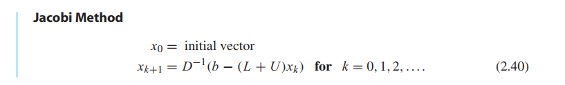
Jacobi Method

The Jacobi Method is a form of 👉Fixed-point Iteration >> for a system of equations.

DEFINITION 2.9
The $n \times n$ matrix $A = (a_{ij})$ is strictly diagonally dominant（严格对角占优） if, for each $1 \leq i \leq n$, $|a_{ii}| > \sum_{j \neq i}|a_{ij} |$. In other words, each main diagonal entry dominates its row in the sense that it is greater in magnitude than the sum of magnitudes of the remainder of the entries in its row.

THEOREM 2.10
If the $n \times n$ matrix $A$ is strictly diagonally dominant, then (1) $A$ is a nonsingular matrix（invertible）, and (2) for every vector $b$ and every starting guess, the Jacobi Method applied to $Ax = b $ converges to the (unique) solution.

Note that strict diagonal dominance is only a sufficient condition. The Jacobi Method may still converge in its absence. (严格的对角占优只是充分条件，没有这个条件Jacobi Method 也可能收敛)

Let $D$ denote the main diagonal of $A$, $L$ denote the lower triangle of $A$ (entries below the main diagonal), and $U$ denote the upper triangle (entries above the main diagonal). Then $A = L + D + U$, and the equation to be solved is $Lx + Dx + Ux = b$.

$$
Ax = b\\
(D + L + U)x = b\\
Dx = b - Lx - Ux\\
x = D^{-1}(b - (L+u)x)
\tag{2.39}
$$

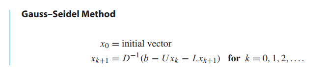
Gauss–Seidel Method and SOR

Gauss–Seidel often converges faster than Jacobi if the method is convergent.

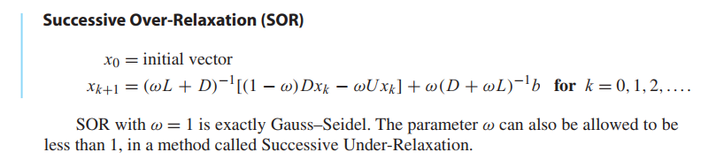
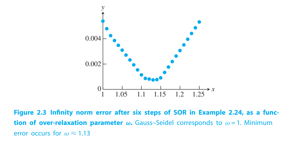
The method called Successive Over-Relaxation (SOR) takes the Gauss–Seidel direction toward the solution and “overshoots” to try to speed convergence. Let $\omega$ be a real number, and define each component of the new guess $x_{k+1}$ as a weighted average of $\omega$ times the Gauss–Seidel formula and $1 - \omega$ times the current guess $x_k$. The number $\omega$ is called the relaxation parameter, and $\omega > 1 $ is referred to as over-relaxation.

💡For example💡:
Apply the Jacobi Method, Gauss-Seidel Method and SOR Method to the system
$$
\begin{cases}
3u + v = 5\\
u + 2v = 5
\end{cases}
$$

Solution:

We use the initial guess $(u_0, v_0) = (0,0)$.
$$
\begin{bmatrix}
3 & 1\\
1 & 2
\end{bmatrix}
\begin{bmatrix}
u \\ v
\end{bmatrix}
=
\begin{bmatrix}
5\\ 5
\end{bmatrix}
$$

• Jacobi Method
  $$
  \begin{aligned}
  \begin{bmatrix}
  u_{k+1} \\ v_{k+1}
  \end{bmatrix}
  &= D^{-1}(b - (L+U)x_k)\\
  &=
  \begin{bmatrix}
  \frac{1}{3} & 0\\
  0 & \frac{1}{2}
  \end{bmatrix}
  (\begin{bmatrix}
  5 \\ 5
  \end{bmatrix} - \begin{bmatrix}
  0 & 1\\ 1 & 0
  \end{bmatrix}\begin{bmatrix}
  u_{k} \\ v_{k}
  \end{bmatrix})\\
  &= \begin{bmatrix}
  (5-v_k)/3\\
  (5-u_k)/2
  \end{bmatrix}
  \end{aligned}
  $$

• Gauss-Seidel Method

$$
\begin{bmatrix}
u_{k+1} \\ v_{k+1}
\end{bmatrix}
=
\begin{bmatrix}
(5-v_k)/3\\
(5-u_{k+1})/2
\end{bmatrix}
$$

• SOR Method

$$
u_{k+1} = (1-\omega)u_k + \omega \frac{5-v_k}{3}\\
v_{k+1} = (1-\omega)v_k + \omega \frac{5-u_{k+1}}{2}
$$

💡For example💡:

Compare Jacobi, Gauss–Seidel, and SOR on the system of six equations in six unknowns:
$$
\begin{bmatrix}
3 & -1 & 0 & 0 & 0 & \frac{1}{2}\\
−1 & 3 & −1 & 0 & \frac{1}{2} & 0\\
0 & −1 & 3 & −1 & 0 & 0\\
0 & 0 & -1 & 3 & -1 & 0\\
0 & \frac{1}{2} & 0 & −1 & 3 & −1\\
\frac{1}{2} & 0 & 0 & 0 & −1 & 3\\
\end{bmatrix}
\begin{bmatrix}
u_1 \\ u_2 \\ u_3 \\ u_4 \\ u_5 \\ u_6
\end{bmatrix}
=
\begin{bmatrix}
\frac{5}{2} \\ \frac{3}{2} \\ 1 \\ 1 \\ \frac{3}{2} \\ \frac{5}{2}
\end{bmatrix}
$$

Solution:

The solution is $x = [1,1,1,1,1,1]$. The approximate solution vectors $x_6$, after running six steps of each of the three methods, are shown in the following table:

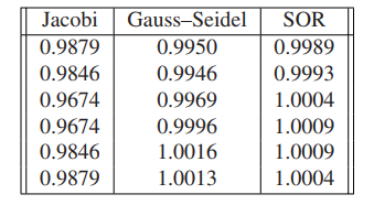
SOR appears to be superior for this problem.

Convergence of iterative methods

to be added…

Sparse matrix computations

A coefficient matrix is called sparse if many of the matrix entries are known to be zero Often, of the $n^2$ eligible entries in a sparse matrix, only $O(n)$ of them are nonzero.

There are two reasons to use iterative methods while Gaussian elimination provide the user a finite number of steps that terminate the solution.

• For real-time applications, suppose that a solution to $Ax = b$ is known, after which $A$ and/or $b$ change by a small amount. In this case, we can iterative from the origin solution, which brings fast convergence. It’s called polish technique.

Gaussian elimination for an $n \times n$ matrix costs on the order of $n^3$ operations.A single step of Jacobi’s Method, for example, requires about $n^2$ multiplications (one for each matrix entry) and about the same number of additions.

• For sparse matrix, Gaussian elimination often brings fill-in, where the coefficient matrix changes from sparse to full due to the necessary row operations. Iterative method can avoid this problem.

💡For example💡:

Use the Jacobi Method to solve the 100,000-equation version of the Example above.

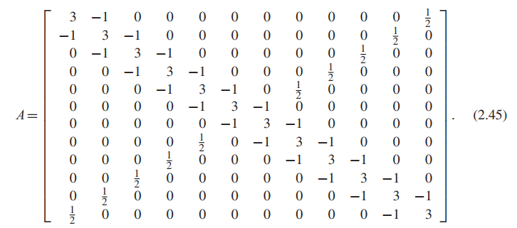
Let $n$ be an even integer, and consider the $n \times n$ matrix $A$ with $3$ on the main diagonal, $−1$ on the super-and subdiagonal, and $1/2$ in the $(i,n + 1 − i)$ position for all $i = 1,…,n$, except for $i = n/2$ and $n/2 + 1$. For $n = 12$,

Define the vector $b = (2.5,1.5, . . . ,1.5,1.0,1.0,1.5, . . . ,1.5,2.5)$, where there are $n − 4$
repetitions of $1.5$ and $2$ repetitions of $1.0$.

Solution:

Since fewer than $4n$ of the potential entries are nonzero, we may call the matrix sparse.

In size, treating the coefficient matrix $A$ as a full matrix means storing $n^2 = 10^{10}$ entries, we need $10^{10} * 8Byte \approx 80GB$ to store this matrix in computer.

In time, $n^3 \approx 10^{15}$, if the machine runs $10^9$ cycles per second, and upper bound on the number of floating point operations per second is around $10^{8}$. Then you need $\frac{10^{15}}{10^{8}} = 10^7$ seconds, and there are $3 \times 10^{7}$ seconds in a year, which means you need $\frac{1}{3}$ year to solve this problem…

On the other hand, one step of an iterative method will require approximately $2 \times 4n = 800,000$ operations. We could do $100$ steps of Jacobi iteration and still finish with fewer than $10^8$ operations, which should take roughly a second or less on a modern PC.

1
2
3
4
5
6
7
8
9
10
11

%sparsesetup.m
% Program 2.1 Sparse matrix setup
% Input: n = size of system
% Outputs: sparse matrix a, r.h.s. b
function [a,b] = sparsesetup(n)
e = ones(n,1); n2=n/2;
a = spdiags([-e 3*e -e],-1:1,n,n); % Entries of a
c=spdiags([e/2],0,n,n);c=fliplr(c);a=a+c;
a(n2+1,n2) = -1; a(n2,n2+1) = -1; % Fix up 2 entries
b=zeros(n,1); % Entries of r.h.s. b
b(1)=2.5;b(n)=2.5;b(2:n-1)=1.5;b(n2:n2+1)=1;

1
2
3
4
5
6
7
8
9
10
11
12
13

%jacobi.m
% Program 2.2 Jacobi Method
% Inputs: full or sparse matrix a, r.h.s. b,
% number of Jacobi iterations, k
% Output: solution x
function x = jacobi(a,b,k)
n=length(b); % find n
d=diag(a); % extract diagonal of a
r=a-diag(d); % r is the remainder
x=zeros(n,1); % initialize vector x
for j=1:k % loop for Jacobi iteration
x = (b-r*x)./d;
end % End of Jacobi iteration loop

1
2
3
4
5
6
7
8
9
10
11
12
13
14
15
16
17
18
19
20
21
22
23
24
25
26
27
28
29
30
31
32
33
34
35
36
37
38
39
40
41
42
43
44
45

>> [a,b] = sparsesetup(6)

a =

   (1,1)       3.0000
   (2,1)      -1.0000
   (6,1)       0.5000
   (1,2)      -1.0000
   (2,2)       3.0000
   (3,2)      -1.0000
   (5,2)       0.5000
   (2,3)      -1.0000
   (3,3)       3.0000
   (4,3)      -1.0000
   (3,4)      -1.0000
   (4,4)       3.0000
   (5,4)      -1.0000
   (2,5)       0.5000
   (4,5)      -1.0000
   (5,5)       3.0000
   (6,5)      -1.0000
   (1,6)       0.5000
   (5,6)      -1.0000
   (6,6)       3.0000


b =

    2.5000
    1.5000
    1.0000
    1.0000
    1.5000
    2.5000

>> jacobi(a,b,40)

ans =

    1.0000
    1.0000
    1.0000
    1.0000
    1.0000
    1.0000

Methods for symmetric positive-definite matrices

Symmetric positive-definite matrices

👉More about Symmetric Matrix >>

DEFINITION 2.12
The $n \times n$ matrixAis symmetric if $A^T = A$. The matrixAis positive-definite if $x^TAx > 0$ for all vectors $x \neq 0$.

Note that a symmetric positive-definite matrix must be nonsingular（invertible）, since it is impossible for a nonzero vector $x$ to satisfy $Ax = 0$.

Property 1
If the $n \times n$ matrix $A$ is symmetric, then $A$ is positive-definite if and only if all of its eigenvalues are positive.

Property 2
If A is $n \times n$ symmetric positive-definite and $X$ is an $n \times m$ matrix of 👉full rank >> with $n \geq m$, then $X^TAX$ is $m × m$ symmetric positive-definite.

DEFINITION 2.13
A principal submatrix of a square matrix $A$ is a square submatrix whose diagonal entries are diagonal entries of $A$.

Property 3
Any principal submatrix of a symmetric positive-definite matrix is symmetric positive definite.(对称正定矩阵的任何主子矩阵都是对称正定矩阵)

Extra Definition
A principal submatrix of a square matrix $A$ is the matrix obtained by deleting any $k$ rows and the corresponding $k$ columns.
The determinant of a principal submatrix is called the principal minor of $A$.

Extra Definition
The leading principal submatrix of order $k$ of an $n \times n$ matrix is obtained by deleting the last $n - k$ rows and column of the matrix.
The determinant of a leading principal submatrix is called the leading principal minor of $A$.

Principal minors can be used in definitess tests

Cholesky factorization

THEOREM 2.14
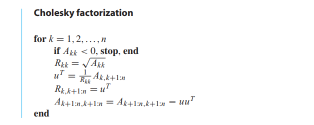
(Cholesky Factorization Theorem) If $A$ is a symmetric positive-definite $n \times n$ matrix, then there exists an upper triangular $n \times n$ matrix $R$ such that $A = R^TR$.

💡For example💡:

Find the Cholesky factorization of
$$
\begin{bmatrix}
4 & -2 & 2\\
-2 & 2 & -4\\
2 & -4 & 11
\end{bmatrix}
$$

Solution:

The top row of $R$ is $R_{11} = \sqrt{a_{11}} = 2$, followed by $u^T = \frac{1}{R_{11}}A_{1,2:3} = [-2,2]/R_{11} = [-1,1]$:
$$
R =
\left[\begin{array}{c:cc}
2 & -1 & 1\\
\hdashline\\
\end{array}\right]
$$
So, $uu^T = \begin{bmatrix}-1 & 1\end{bmatrix} \begin{bmatrix}-1\\1\end{bmatrix}$.

The lower principle $2 \times 2$ submatrix $A_{2:3,2:3}$ of $A$ is
$$
\left[\begin{array}{c:cc}
& & &\\
\hdashline
& 2 & -4 \\
& -4 & 11
\end{array}\right]
-
\left[\begin{array}{c:cc}
& & &\\
\hdashline
& 1 & -1 \\
& -1 & 1
\end{array}\right]
=
\left[\begin{array}{c:cc}
& & &\\
\hdashline
& 1 & -3 \\
& -3 & 10
\end{array}\right]
$$
Now we repeat the same steps on the $2 \times 2$ submatrix to find $R_{22} = 1$ and $R_{23} = −3/1=−3$:
$$
R = \left[\begin{array}{c:cc}
2 & -1 & 1\\
\hdashline
& 1 & -3\\
\end{array}\right]
$$
The lower $1 \times 1$ principal submatrix of $A$ is $10 − (−3)(−3) = 1$, so $R_{33} = \sqrt 1$. The Cholesky factor of $A$ is
$$
R = \left[\begin{array}{ccc}
2 & -1 & 1\\
0 & 1 & -3\\
0 & 0 & 1
\end{array}\right]
$$

Conjugate Gradient Method（共轭梯度法）

DEFINITION 2.15
Let $A$ be a symmetric positive-definite $n \times n$ matrix. For two $n$-vectors $v$ and $w$, define the $A$-inner product
$$
(v,w)_A = v^TAw
$$
The vectors $v$ and $w$ are $A$-conjugate if $(v,w)_A = 0$.

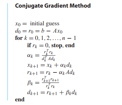
The vector $x_k$ is the approximate solution at step $k$. The vector $r_k$ represents the residual of the approximate solution $x_k$. The vector $d_k$ represents the new search direction used to update the approximation $x_k$ to the improved version $x_{k+1}$.

THEOREM 2.16
Let $A$ be a symmetric positive-definite $n \times n$ matrix and let $b \neq 0$ be a vector. In the Conjugate Gradient Method, assume that $r_k \neq 0$ for $k < n$ (if $r_k = 0$ the equation is solved). Then for each $1 \leq k \leq n$,
(a) The following three subspaces of $R^n$ are equal: $<x_1, . . . , x_k> = <r_0, . . . , r_{k−1}> = <d_0, . . . , d_{k−1}>$
(b) the residuals $r_k$ are pairwise orthogonal: $r^T_k r_j = 0$ for $j < k$,
(c) the directions $d_k$ are pairwise $A$-conjugate: $d^T_k A d_j = 0$ for $j < k$.

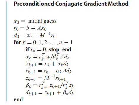
Preconditioning

Nonlinear Systems of Equations

This section describes Newton’s Method and variants for the solution of systems of nonlinear equations.

Multivariate Newton’s Method

One-variable Newton’s Method is
$$
f(x) = 0\\
x_{k+1} = x_k - \frac{f(x)}{f’(x_k)}
$$

Let

$$
f_1(u,v,w) = 0\\
f_2(u,v,w) = 0\\
f_3(u,v,w) = 0\\
\tag{2.49}
$$
be three nonlinear equations in three unknowns $u,v,w$.

Define the vector-valued function $F(u,v,w) = (f_1, f_2,f_3)$. The analogue of the derivative $f’$ in the one-variable case is the Jacobian matrix defined by

$$
DF(x) =
\begin{bmatrix}
\frac{\partial f_1}{\partial u} & \frac{\partial f_1}{\partial v} & \frac{\partial f_1}{\partial w}\\
\frac{\partial f_2}{\partial u} & \frac{\partial f_2}{\partial v} & \frac{\partial f_2}{\partial w}\\
\frac{\partial f_3}{\partial u} & \frac{\partial f_3}{\partial v} & \frac{\partial f_3}{\partial w}
\end{bmatrix}
$$

The Taylor expansion for vector-valued functions around $x_0$ is

$$
F(x) = F(x_0) + DF(x_0) \cdot (x - x_0) + O(x - x_0)^2
$$

Newton’s Method is based on a linear approximation, ignoring the $O(x^2)$ terms.

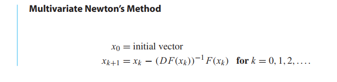
Since computing inverses is computationally burdensome, we use a trick to avoid it.

Set $x_{k+1} = x_k − s$, where s is the solution of $DF(x_k)s = F(x_k)$. Now, only Gaussian elimination ($n^3/3$ multiplications) is needed to carry out a step, instead of computing an inverse (about three times as many).

$$
\begin{cases}
DF(x_k)s = -F(x_k)\\
x_{k+1} = x_k + s
\end{cases}
\tag{2.51}
$$

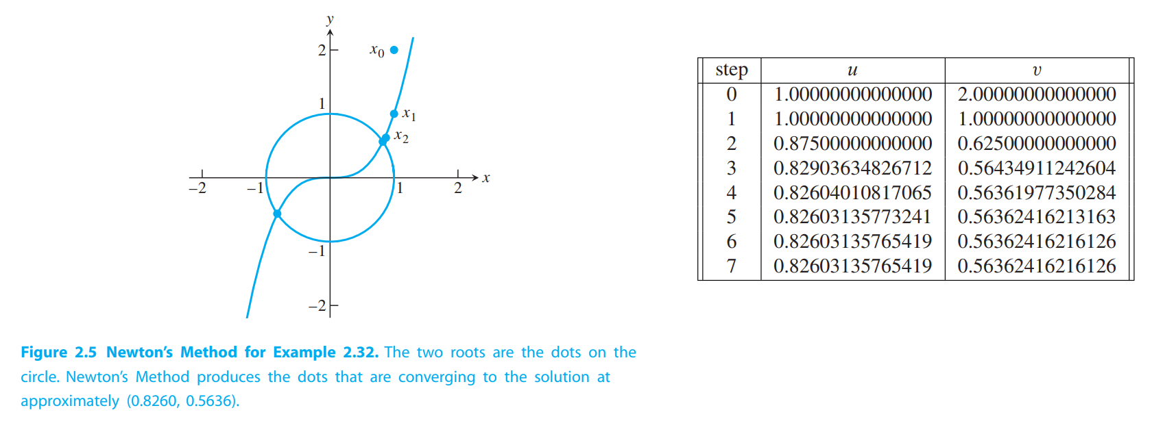
💡For example💡:

Use Newton’s Method with starting guess $(1,2)$ to find a solution of the system
$$
\begin{cases}
v - u^3 = 0\\
u^2 + v^2 - 1= 0
\end{cases}
$$

Solution:

The Jacobian matrix is
$$
DF(u,v) =
\begin{bmatrix}
-3u^2 & 1\\
2u & 2v
\end{bmatrix}
$$
Using starting point $x_0 = (1,2)$, on the first step we must solve the matrix equation (2.51):

$$
\begin{bmatrix}
-3 & 1\\
2 & 4
\end{bmatrix}
\begin{bmatrix}
s_1\\s_2
\end{bmatrix}
=
-\begin{bmatrix}
1\\4
\end{bmatrix}
$$
The solution is s = $(0,−1)$, so the first iteration produces $x_1 = x_0 + s = (1,1)$. The second
step requires solving

$$
\begin{bmatrix}
-3 & 1\\
2 & 2
\end{bmatrix}
\begin{bmatrix}
s_1\\s_2
\end{bmatrix}
=
-\begin{bmatrix}
0\\1
\end{bmatrix}
$$

…

Broyden’s Method

Newton’s Method is a good choice if the Jacobian can be calculated. If not, the best alternative is Broyden’s Method.

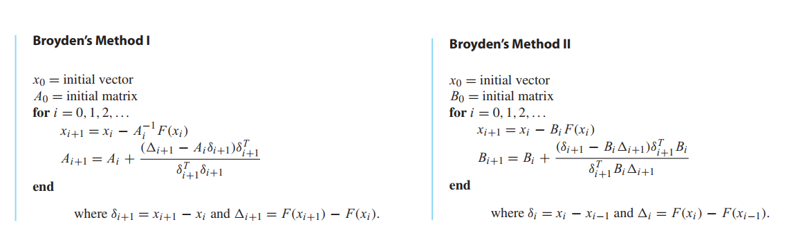
Suppose $A_i$ is the best approximation available at step $i$ to the Jacobian matrix, and that it has been used to create
$$
x_{i+1} = x_i - A_i^{-1}F(x_i)
\tag{2.52}
$$
To update $A_i$ to $A_{i+1}$ for the next step, we would like to respect the derivative aspect of the Jacobian $DF$（从导数的定义出发）, and satisfy
$$
A_{i+1}\delta_{i+1} = \Delta_{i+1}
\tag{2.53}
$$
where, $\delta_{i+1} = x_{i+1} - x_i$ and $\Delta_{i+1} = F(x_{i+1}) - F(x_{i})$.

= = Don’t understand.. = =

On the other hand, for the 👉orthogonal complement(正交补) >> of $\delta_{i+1}$, we have no new information. Therefore, we ask that
$$
A_{i+1}w = A_i w
\tag{2.54}
$$
for every $w$ satisfying (why?)
$$
\delta_{i+1}^T w = 0
$$
One checks that a matrix that satisfies both (2.53) and (2.54) is
$$
A_{i+1} = A_i + \frac{(\Delta_{i+1} - A_i \delta_i)\delta_{i+1}^T}{\delta_{i+1}^T\delta_{i+1}}
\tag{2.55}
$$
Broyden’s Method uses the Newton’s Method step (2.52) to advance the current guess, while updating the approximate Jacobian by (2.55).