PatterRecognition-C1-Introduction

Keywords: Bayes’Theorem, Polynomial Curve Fitting, Posterior Probability, Python

This is the Chapter1 ReadingNotes from book Bishop-Pattern-Recognition-and-Machine-Learning-2006. [Code_Python]

Cases such as the digit recognition example, in which the aim is to assign each input vector to one of a finite number of discrete categories, are called classification problems.

If the desired output consists of one or more continuous variables, then the task is called regression.

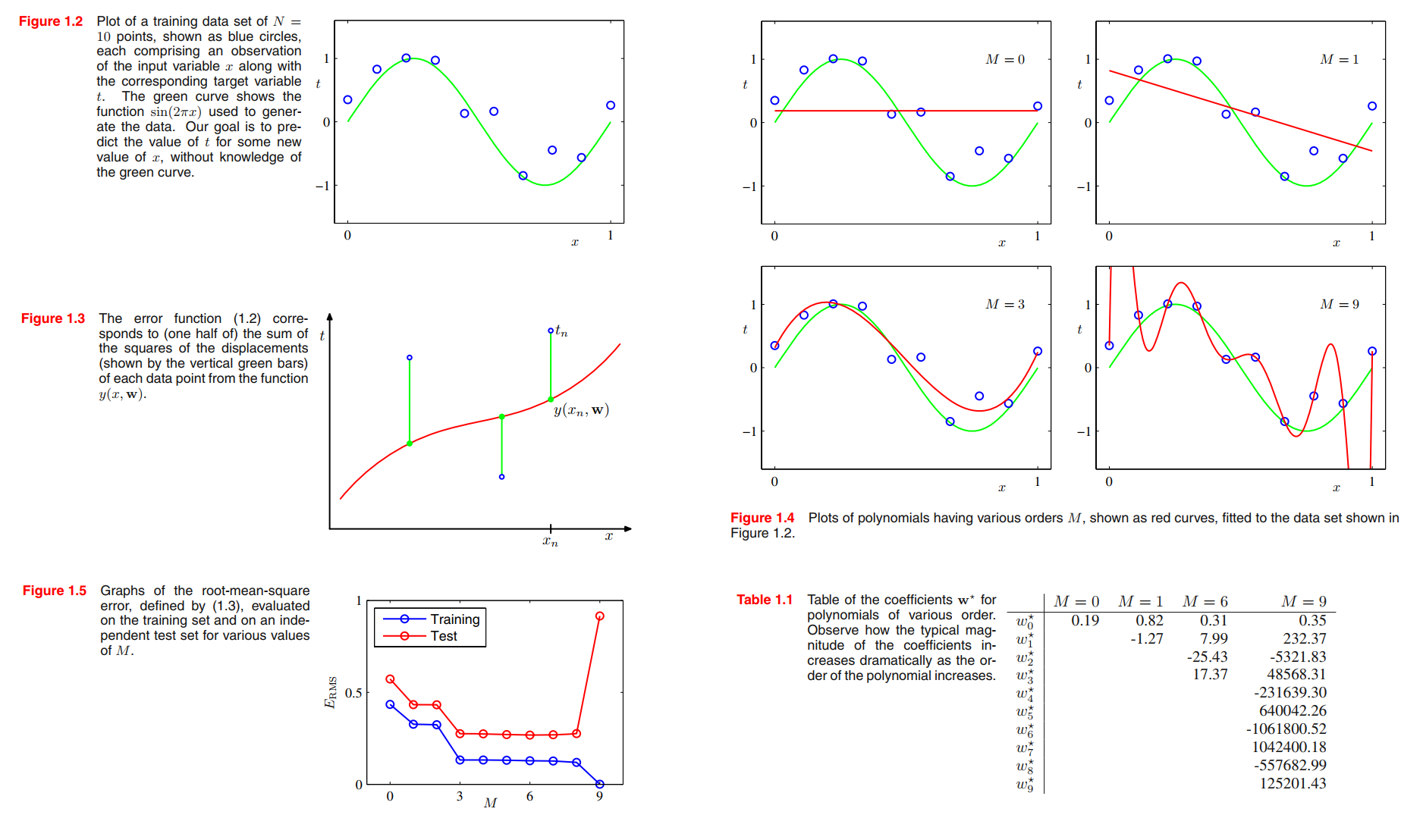
Example: Polynomial Curve Fitting(error minimization view)

👉More about Polynomial Curve Fitting in Numerical Analysis >>

$$
y(x,\pmb{w}) = w_0 + w_1 x + \cdots + w_Mx^M = \sum_{j=0}^{M}w_jx^j
\tag{1.1}
$$
Note that, although the polynomial function $y(x,\pmb{w})$ is a nonlinear function of $x$, it is a linear function of the coefficients $\pmb{w}$. Functions, such as the polynomial, which are linear in the unknown parameters have important properties and are called linear models and will be discussed extensively in Chapters 3 and 4.

$$
E(\pmb{w}) = \frac{1}{2}\sum_{n=1}^{N}\lbrace y(x_n, \pmb{w}) - t_n\rbrace ^ 2
\tag{1.2}
$$

Because the error function is a quadratic function of the coefficients $\pmb{w}$, its derivatives with respect to the coefficients will be linear in the elements of $\pmb{w}$, and so the minimization of the error function has a unique solution, denoted by $\pmb{w}^{\ast}$, which can be found in closed form.

$$
E_{RMS} = \sqrt{2E(\pmb{w^{\ast}})/N}
\tag{1.3}
$$

the fitted curve oscillates wildly and gives a very poor representation of the function sin(2πx). This latter behaviour is known as over-fitting.

We shall see that the least squares approach to finding the model parameters represents a specific case of maximum likelihood (discussed in Section 1.2.5), and that the over-fitting problem can be understood as Section 3.4 a general property of maximum likelihood. By adopting a Bayesian approach, the over-fitting problem can be avoided.

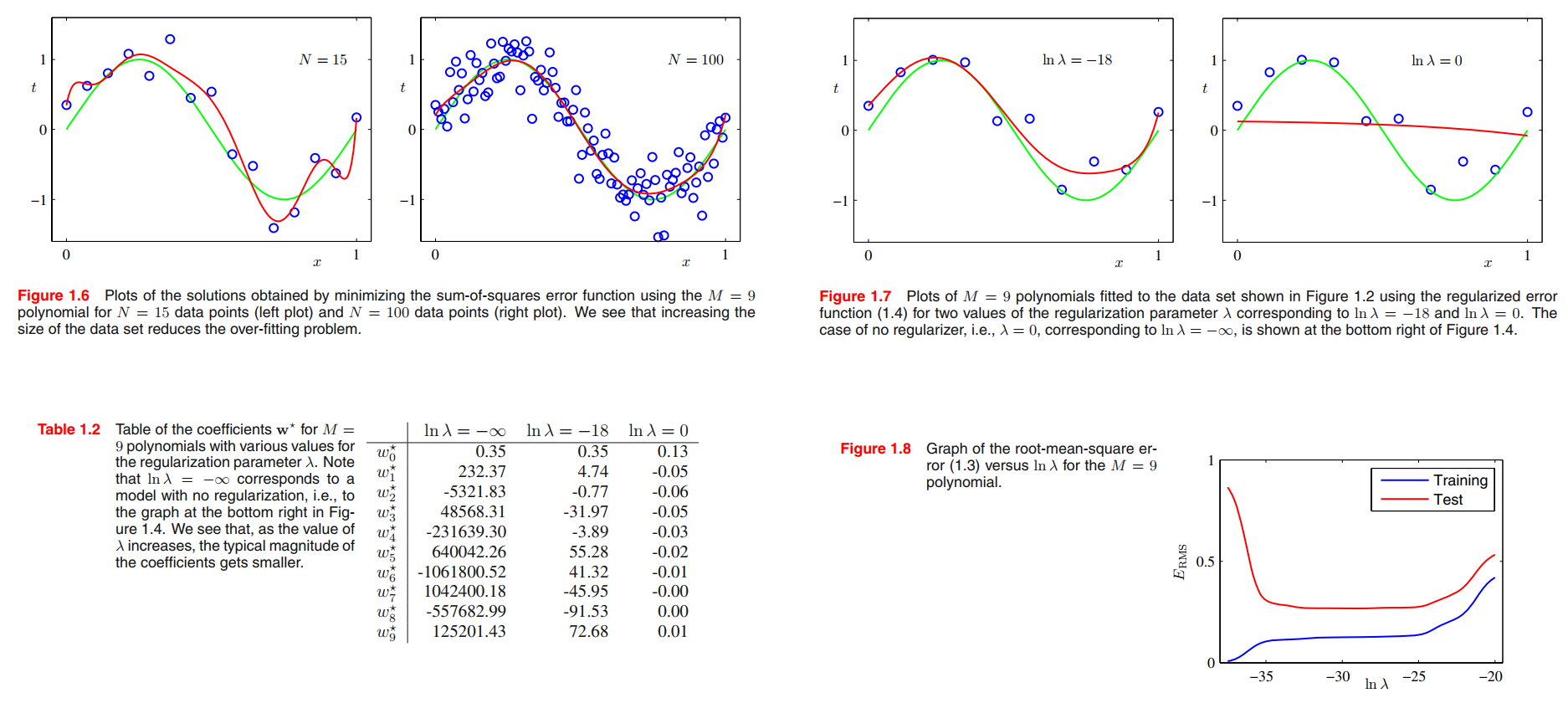
One technique that is often used to control the over-fitting phenomenon in such cases is that of regularization, which involves adding a penalty term to the error function (1.2) in order to discourage the coefficients from reaching large values.
$$
\tilde{E}{(\pmb{w})} = \frac{1}{2}\sum_{n=1}^{N}\lbrace y(x_n, \pmb{w}) - t_n\rbrace ^ 2 + \frac{\lambda}{2}||\pmb{w}||^2
\tag{1.4}
$$

by taking the available data and partitioning it into a training set, used to determine the coefficients $\pmb{w}$, and a separate validation set, also called a hold-out set, used to optimize the model complexity (either $M$ or $\lambda$).

Probability Theory

the identity of the box that will be chosen is a random variable, which we shall denote by $B$. This random variable can take one of two possible values, namely $r$ (corresponding to the red box) or $b$ (corresponding to the blue box).

the identity of the fruit is also a random variable and will be denoted by $F$. It can take either of the values $a$ (for apple) or $o$ (for orange).

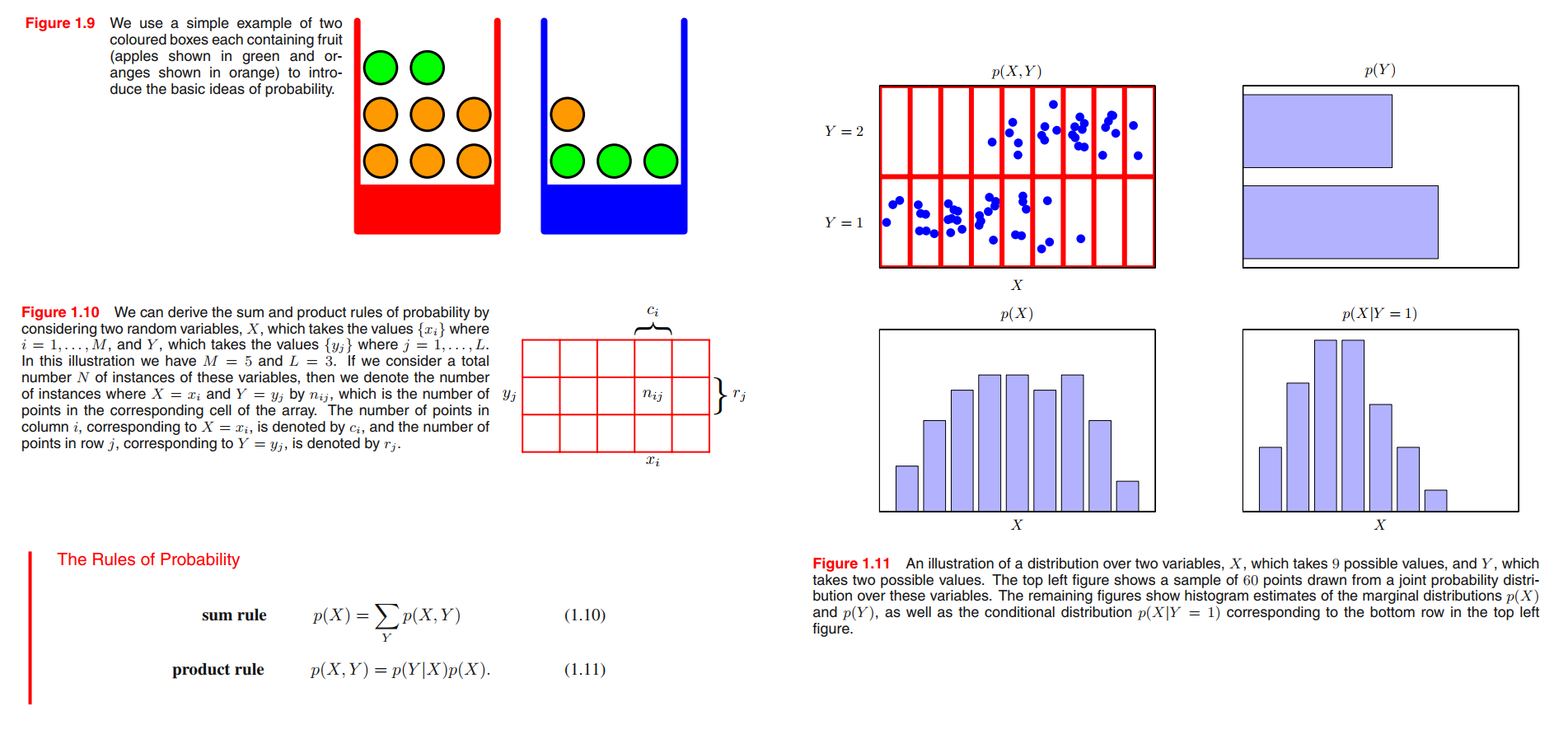
See Figure 1.10, two random variables $X$ and $Y$ (which could for instance be the Box and Fruit variables considered above).A total of N trials in which we sample both of the variables $X$ and $Y$.

the joint probability of $X = x_i$ and $Y = y_j$ is
$$
p(X=x_i, Y = y_j) = \frac{n_{ij}}{N}
\tag{1.5}
$$
Here we are implicitly considering the $limit N \rightarrow \infty$.

the marginal probability is,
$$
\begin{aligned}
p(X = x_i) &= \frac{c_i}{N}\\ &= \sum_{j=1}^Lp(X=x_i,Y=y_j)
\end{aligned}
\tag{1.7}
$$

the conditional probability is,
$$
p(Y=y_j | X= x_i) = \frac{n_{ij}}{c_i}
\tag{1.8}
$$

thus,

$$
\begin{aligned}
p(X = x_i, Y = y_j) &= \frac{n_{ij}}{N}\\
&= \frac{n_{ij}}{c_i} \cdot \frac{c_i}{N} \\
&= p(Y=y_j | X= x_i) p(X = x_i)
\end{aligned}
\tag{1.9}
$$

From the product rule, together with the symmetry property $p(X, Y) = p(Y,X)$, we immediately obtain the following relationship between conditional probabilities, which is called Bayes’theorem
$$
p(Y|X) = \frac{p(X|Y)p(Y)}{p(X)}
\tag{1.12}
$$

Using the sum rule, the denominator in Bayes’ theorem can be expressed in terms of the quantities appearing in the numerator
$$
p(X) = \sum_{Y}p(X|Y)p(Y)
\tag{1.13}
$$

Now back to box and fruit,

$$
p(B=r) = \frac{4}{10}, p(B=b) = \frac{6}{10}
$$
$$
p(F = a | B = r) = \frac{1}{4}\\
p(F = o | B = r) = \frac{3}{4}\\
p(F = a | B = b) = \frac{3}{4}\\
p(F = o | B = b) = \frac{1}{4}
$$

note that these probabilities are normalized so that
$$
p(F=a|B=r) + p(F=o|B=r) = 1\\
p(F=a|B=b) + p(F=o|B=b) = 1
$$

We can now use the sum and product rules of probability to evaluate the overall probability of choosing an apple
$$
\begin{aligned}
p(F = a) &= p(F=a|B=r)p(B=r) + p(F=a|B=b)p(B=b)\\
&= \frac{1}{4} \times \frac{4}{10} + \frac{3}{4} \times \frac{6}{10}\\
&=\frac{11}{20}\\
p(F=o) &=1-\frac{11}{20} = \frac{9}{20}
\end{aligned}
\tag{1.22}
$$

We can solve the problem of reversing the conditional probability by using Bayes’ theorem to give

$$
\begin{aligned}
p(B=r|F=o) &= \frac{p(F=o|B=r)p(B=r)}{p(F=o)}\\
&= \frac{3}{4}\times \frac{4}{10} \times \frac{20}{9}\\
&=\frac{2}{3}
\end{aligned}
\tag{1.23}
$$

1. If we had been asked which box had been chosen before being told the identity of the selected item of fruit, then the most complete information we have available is provided by the probability $p(B)$. We call this the prior probability because it is the probability available before we observe the identity of the fruit.
2. Once we are told that the fruit is an orange, we can then use Bayes’ theorem to compute the probability $p(B|F)$, which we shall call the posterior probability because it is the probability obtained after we have observed $F$.
3. Bayes’ theorem was used to convert a prior probability into a posterior probability by incorporating the evidence provided by the observed data.

Probability densities

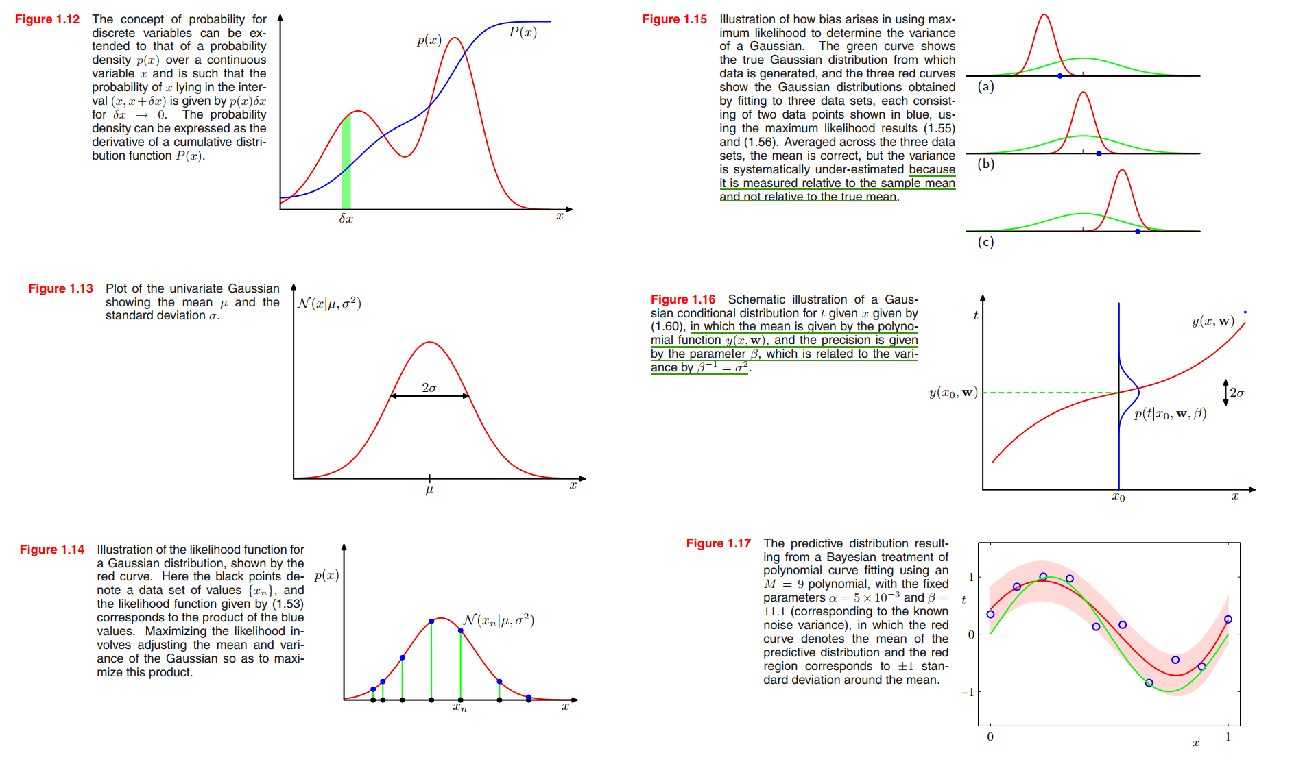
If the probability of a real-valued variable $x$ falling in the interval $(x, x + \sigma x)$ is given by $p(x)\sigma x$ for $\sigma x \rightarrow 0$, then $p(x)$ is called the probability density over $x$.
$$
p(x\in(a,b)) = \int_a^b p(x) dx
\tag{1.24}
$$
$$
p(x) \geq 0 \tag{1.25}
$$
$$
\int_{-\infty}^{\infty} p(x)dx = 1 \tag{1.26}
$$
$$
P(z) = \int_{-\infty}^{z} p(x) dx\tag{1.28}
$$

Expectations and covariances

The average value of some function $f(x)$ under a probability distribution $p(x)$ is called the expectation of $f(x)$ and will be denoted by $E[f]$.

$$
E[f] = \sum_{x} p(x) f(x)
\tag{1.33}
$$

$$
E[f] = \int p(x)f(x) dx
\tag{1.34}
$$

The variance of $f(x)$ is
$$
\begin{aligned}
var[f] &= E[(f(x) - E[f(x)])^2]\\
&= E[f(x)^2] - E[f(x)]^2
\end{aligned}
\tag{1.38}
$$
and provides a measure of how much variability there is in $f(x)$ around its mean value $E[f(x)]$.

conditional expectation for two-variable function $f(x,y)$:

$$
E_x[f|y] = \sum_x p(x|y)f(x)
\tag{1.37}
$$

For two random variables $x$ and $y$, the covariance is defined by

$$
\begin{aligned}
cov[x,y]&= E_{x,y}[\lbrace x - E(x)\rbrace \lbrace y - E(y)\rbrace] \\
&= E_{x,y}[xy] - E[x]E[y]
\end{aligned}
\tag{1.41}
$$
expresses the extent to which $x$ and $y$ vary together. If $x$ and $y$ are independent, then their covariance vanishes.

In the case of two vectors of random variables $\pmb{x}$ and $\pmb{y}$, the covariance is a matrix(默认是列向量)

$$
\begin{aligned}
cov[\pmb{x},\pmb{y}]&= E_{\pmb{x,y}}[\lbrace \pmb{x} - E(\pmb{x})\rbrace \lbrace \pmb{y^T} - E(\pmb{y^T})\rbrace] \\
&= E_{\pmb{x,y}}[\pmb{xy^T}] - E[\pmb{x}]E[\pmb{y^T}]
\end{aligned}
\tag{1.42}
$$

Bayesian probabilities

Two ways to see probability:

• frequentist interpretation. view probabilities in terms of the frequencies of random, repeatable events.

• Bayesian view. probabilities provide a quantification of uncertainty.(不确定性的量化)

we can adopt a similar approach (fruit in boxes) when making inferences about quantities such as the parameters $\pmb{w}$ in the polynomial curve fitting example.

1. We capture our assumptions about $\pmb{w}$, before observing the data, in the form of a prior probability distribution $p(\pmb{w})$.
2. The effect of the observed data $D = {t_1, \cdots, t_N}$ is expressed through the conditional probability $p(D|\pmb{w})$
3. Bayes’ theorem, which takes the form
   $$
   p(\pmb{w}|D) = \frac{p(D|\pmb{w})p(\pmb{w})}{p(D)}
   \tag{1.43}
   $$
4. then allows us to evaluate the uncertainty in $\pmb{w}$ after we have observed $D$ in the form of the posterior probability $p(\pmb{w}|D)$.

The quantity $p(D|\pmb{w})$ on the right-hand side of Bayes’ theorem is evaluated for the observed data set $D$ and can be viewed as a function of the parameter vector $\pmb{w}$, in which case it is called the likelihood function. It expresses how probable the observed data set is for different settings of the parameter vector $\pmb{w}$.

$$
posterior \propto likelihood \times prior
\tag{1.44}
$$

Indeed, integrating both sides of (1.43) with respect to $\pmb{w}$, we can express the denominator in Bayes’ theorem in terms of the prior distribution and the likelihood function
$$
p(D) = \int p(D|\pmb{w})p(\pmb{w}) d\pmb{w}
\tag{1.45}
$$
where, $\int p(\pmb{w}|D) d \pmb{w} = 1$.

The Gaussian distribution

For the case of a single real-valued variable $x$, the Gaussian distribution is defined by
$$
\mathcal{N}(x | \mu, \sigma^2) = \frac{1}{(2\pi \sigma^2)^{\frac{1}{2}}} exp\lbrace -\frac{1}{2\sigma^2}(x-\mu)^2\rbrace
\tag{1.46}
$$
which is governed by two parameters: $\mu$, called the mean, and $\sigma^2$, called the variance, the reciprocal of the variance, written as $\beta = \frac{1}{\sigma^2}$, is called the precision.

$$
\int_{-\infty}^{\infty} \mathcal{N}(x|\mu, \sigma^2)aligned dx = 1
\tag{1.48}
$$

We are also interested in the Gaussian distribution defined over a $D$-dimensional vector $\pmb{x}$ of continuous variables, which is given by
$$
\mathcal{N}(\pmb{x} | \pmb{\mu}, \pmb{\Sigma}) = \frac{1}{(2\pi)^{D/2}}\frac{1}{|\pmb{\Sigma}|^{1/2}} exp \lbrace -\frac{1}{2}(\pmb{x - \mu})^T \pmb{\Sigma}^{-1}(\pmb{x-\mu}) \rbrace
\tag{1.52}
$$
where $\pmb{\Sigma}$ is a $D \times D$ matrix, called : covariance.

1. Now suppose that we have a data set of observations $X = (x_1, \cdots , x_N)^T$, representing $N$ observations of the scalar variable $x$.
2. We shall suppose that the observations are drawn independently from a Gaussian distribution whose mean $\mu$ and variance $\sigma^2$ are unknown, and we would like to determine these parameters from the data set.
3. Because our data set $X$ is i.i.d., we can therefore write the probability of the data set, given mean $\mu$ and variance $\sigma^2$, in the form
   $$
   p(X|\mu, \sigma^2) = \prod_{n=1}^{N} \mathcal{N}(x_n|\mu, \sigma^2)
   \tag{1.53}
   $$
4. When viewed as a function of mean $\mu$ and variance $\sigma^2$, this is the likelihood function for the Gaussian and is interpreted diagrammatically in Figure 1.14.
5. We shall determine values for the unknown parameters $\mu$ and $\sigma^2$ in the Gaussian by maximizing the likelihood function (1.53). it is convenient to maximize the logarithm of the likelihood function.
   $$
   \ln p(X|\mu, \sigma^2) = -\frac{1}{2\sigma^2} \sum_{n=1}^{N} (x_n - \mu)^2 - \frac{N}{2} \ln \sigma^2 - \frac{N}{2}\ln(2\pi)
   \tag{1.54}
   $$
6. Maximizing (1.54) with respect to $\mu$, we get sample mean.
   $$
   \mu_{ML} = \frac{1}{N} \sum_{n=1}^N x_n
   \tag{1.55}
   $$
7. Maximizing (1.54) with respect to $\sigma^2$, we get sample variance.
   $$
   \sigma^2_{ML} = \frac{1}{N}\sum_{n=1}^N (x_n - \mu_{ML})^2
   \tag{1.56}
   $$
8. In particular, we shall show that the maximum likelihood approach systematically underestimates the variance of the distribution. The following estimate for the variance parameter is unbiased(无偏估计)
   $$
   \widetilde{\sigma^2} = \frac{N}{N-1}\sigma_{ML}^2 = \frac{N}{N-1}\sum_{n=1}^N (x_n - \mu_{ML})^2
   \tag{1.59}
   $$
9. 👉Why underestimates? >>

Curve fitting re-visited(probabilistic perspective)

1. The goal in the curve fitting problem is to be able to make predictions for the target variable $t$ given some new value of the input variable $x$ on the basis of a set of training data comprising $N$ input values $X = (x_1, \cdots , x_N)^T$ and their corresponding target values $T = (t_1, \cdots , t_N)^T$.
2. We can express our uncertainty over the value of the target variable using a probability distribution.
3. For this purpose, we shall assume that, given the value of $x$, the corresponding value of $t$ has a Gaussian distribution with a mean equal to the value $y(x,\pmb{w})$ of the polynomial curve given by (1.1). Thus we have(See Figure 1.16.)
   $$
   p(t|x,\pmb{w}, \beta) = \mathcal{N}(t|y(x,\pmb{w}), \beta^{-1}) \tag{1.60}
   $$
4. We now use the training data $\lbrace X,T \rbrace$ to determine the values of the unknown parameters $\pmb{w}$ and $\pmb{β}$ by maximum likelihood. If the data are assumed to be drawn independently from the distribution (1.60), then the likelihood function is given by
   $$
   p(T|X, \pmb{w}, \beta) = \prod_{n=1}^N \mathcal{N}(t_n | y(x_n, \pmb{w}), \beta^{-1})
   \tag{1.61}
   $$
5. log function is convienient.
   $$
   \ln p(T|X, \pmb{w}, \beta) = -\frac{\beta}{2}\sum_{n=1}^N\lbrace y(x_n, \pmb{w}) - t_n \rbrace^2 + \frac{N}{2} \ln \beta - \frac{N}{2} \ln(2\pi)
   \tag{1.62}
   $$
6. maximum the (1.62) with respect to $\mu$, We therefore see that maximizing likelihood is equivalent, so far as determining $\pmb{w}$ is concerned, to minimizing the sum-of-squares error function defined by (1.2).
7. maximum the (1.62) with respect to $\beta$,
   $$
   \frac{1}{\beta_{ML}} = \frac{1}{N}\sum_{n=1}^{N} \lbrace y(x_n, \pmb{w_{ML}}) - t_n\rbrace^2
   \tag{1.63}
   $$
8. Having determined the parameters $\pmb{w}$ and $\pmb{β}$, we can now make predictions for new values of $x$. Because we now have a probabilistic model, these are expressed in terms of the predictive distribution that gives the probability distribution over $t$, rather than simply a point estimate, and is obtained by substituting the maximum likelihood parameters into (1.60) to give
   $$
   p(t|x, \pmb{w_{ML}}, \beta_{ML}) = \mathcal{N}(t|y(x, \pmb{w_{ML}}), \beta_{ML}^{-1})
   \tag{1.64}
   $$
9. Let us introduce a prior distribution over the polynomial coefficients $\pmb{w}$. Let us consider a Gaussian distribution of the form
   $$
   p(\pmb{w}|\alpha) = \mathcal{N}(\pmb{w}| \pmb{0}, \alpha^{-1} \pmb{I}) = (\frac{\alpha}{2\pi})^{(M+1)/2} exp \lbrace -\frac{\alpha}{2} \pmb{w}^T\pmb{w}\rbrace
   \tag{1.65}
   $$
   where $\alpha$ is the precision of the distribution, and $M+1$ is the total number of elements in the vector $\pmb{w}$ for an $M$th order polynomial. Variables such as $\alpha$, which control the distribution of model parameters, are called hyperparameters.
10. Using Bayes’ theorem, the posterior distribution for $\pmb{w}$ is proportional to the product of the prior distribution and the likelihood function
    $$
    p(\pmb{w}|X,T,\alpha, \beta) \propto p(T|X,\pmb{w}, \beta) p(\pmb{w}|\alpha)
    \tag{1.66}
    $$
11. We can now determine $\pmb{w}$ by finding the most probable value of $\pmb{w}$ given the data, in other words by maximizing the posterior distribution. This technique is called maximum posterior, or simply MAP.
12. By(1.62), (1.65) and (1.66), we find that the maximum of the posterior is given by the minimum of
    $$
    \frac{\beta}{2} \sum_{n=1}^{N}\lbrace y(x_n, \pmb{w}) - t_n\rbrace^2 + \frac{\alpha}{2}\pmb{w^T}\pmb{w}
    \tag{1.67}
    $$
13. Thus we see that maximizing the posterior distribution is equivalent to minimizing the regularized sum-of-squares error function encountered earlier in the form (1.4), with a regularization parameter given by $\lambda = \frac{\alpha}{\beta}$.

Bayesian curve fitting(using integration)

In a fully Bayesian approach, we should consistently apply the sum and product rules of probability, which requires, as we shall see shortly, that we integrate over all values of $\pmb{w}$.

In the curve fitting problem, we are given the training data $X$ and $T$, along with a new test point $x$, and our goal is to predict the value of $t$. We therefore wish to evaluate the predictive distribution $p(t|x, X, T)$.

$$
p(t|x,X,T) = \int \underbrace{p(t|x,\pmb{w})}_{(1.60)}
\underbrace{p(\pmb{w}|X,T)}_{post-distribution(1.66)}d\pmb{w}
\tag{1.68}
$$

The integration in (1.68) can also be performed analytically with the result that the predictive distribution is given by a Gaussian of the form
$$
p(t|x,X,T) = \mathcal{N}(t|m(x),s^2(x))
\tag{1.69}
$$
where the mean and variance are given by
$$
m(x) = \beta \phi(x)^T S\sum_{n=1}^{N} \phi(x_n)t_n
\tag{1.70}
$$
$$
s^2(x) = \beta^{-1} + \phi(x)^TS\phi(x)
\tag{1.71}
$$
where, the matrix $S$ is given by
$$
S^{-1} = \alpha \pmb{I} + \beta \sum_{n=1}^{N} \phi(x_n)\phi(x)^T
\tag{1.72}
$$
where $\pmb{I}$ is the unit matrix, and we have defined the vector $\phi(x)$ with elements $\phi_i(x) = x^i, for, i = 0, \cdots , M$.

Model Selection

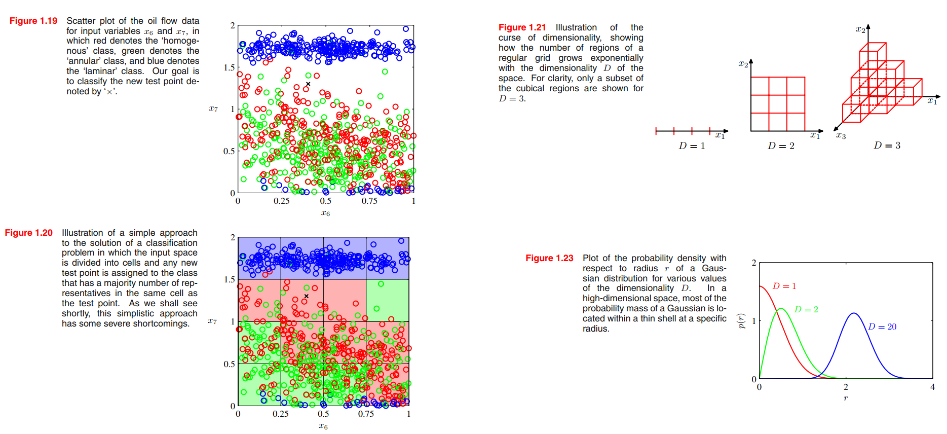
The Curse of Dimensionality

Decision Theory

Minimizing the misclassification rate

Minimizing the expected loss

The reject option

Inference and decision

Loss functions for regression

Information Theory

Relative entropy and mutual information