NumericalAnalysis-C3-Interpolation

Keywords: Lagrange interpolation, Chebyshev Interpolation, Cubic Splines, Bézier Curves, Mathlab

This is the Chapter3 ReadingNotes from book Numerical Analysis by Timothy.

👉First Understanding about Interpolation and Curves>>

Data and Interpolating Functions

DEFINITION 3.1
The function $y = P(x)$ interpolates the data points $(x_1,y_1), \cdots , (x_n,y_n)$ if $P(x_i) = y_i$ for each $1 \leq i \leq n$.

No matter how many points are given, there is some polynomial $y = P(x)$ that runs through all the points.

Lagrange interpolation

THEOREM 3.2
Main Theorem of Polynomial Interpolation. Let $(x_1,y_1), . . . , (x_n,y_n)$ be $n$ points in the plane with distinct $x_i$. Then there exists one and only one polynomial $P$ of degree $n − 1$ or less that satisfies $P(x_i) = y_i$ for $i = 1,…,n$.

Newton’s divided differences（牛顿分差法）

DEFINITION 3.3
Denote by $f[x_1 . . . x_n]$ the coefficient of the $x^{n−1}$ term in the (unique) polynomial that interpolates $(x_1,f(x_1)), . . . , (x_n,f(x_n))$.

💡For example💡:

Find an interpolating polynomial for the data points $(0,1), (2,2)$, and $(3,4)$ in Figure 3.1.

Solution:

By Lagrange’s formula:

$$
P_2(x) = \frac{1}{2}x^2 - \frac{1}{2}x + 1
$$

Check that $P_2(0) = 1,P_2(2) = 2$, and $P_2(3) = 4$.

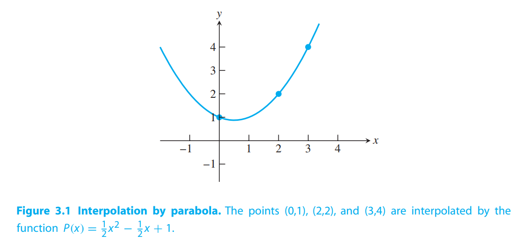
Thus, by definition 3.3
$$
f[0 \space 2 \space3] = \frac{1}{2}
$$

Using this definition, the following somewhat remarkable alternative formula for the interpolating polynomial holds, called the Newton’s divided difference formula

$$
\begin{aligned}
P(x) = f[x_1] &+ f[x_1 x_2](x - x_1) \\
&+ f[x_1 x_2 x_3](x - x_1)(x - x_2)\\
&+ \cdots \\
&+ f[x_1 x_2 \cdots x_n](x - x_1)(x-x_2)\cdots(x - x_{n-1})
\end{aligned}
\tag{3.2}
$$
and it’s easy to calculate
$$
\begin{aligned}
&f[x_k] = f(x_k)\\
&f[x_k x_{k+1}] = \frac{f[x_{k+1}]-f[x_k]}{x_{k+1} - x_{k}}\\
&f[x_k x_{k+1} x_{k+2}] = \frac{f[x_{k+1} x_{k+2}] - f[x_k x_{k+1}]}{x_{k+2} - x_{k}}\\
&f[x_k x_{k+1} x_{k+2} x_{k+3}] = \frac{f[x_{k+1} x_{k+2} x_{k+3}] - f[x_k x_{k+1} x_{k+2}]}{x_{k+3} - x_{k}}\\
\end{aligned}
\tag{3.3}
$$

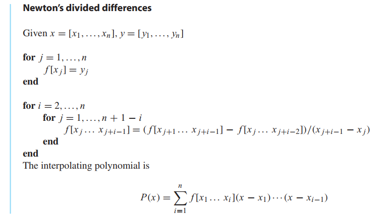
For three points the table has the form(convenient to understand)

The divided difference approach has a “real-time updating’’ property that the Lagrange form lacks: The Lagrange polynomial must be restarted from the beginning when a new point is added; none of the previous calculation can be used; in divided difference form, we keep the earlier work and add one new term to the polynomial.

How many degree d polynomials pass through n points?

Code for interpolation

1
2
3
4
5
6
7
8
9
10
11
12
13
14
15
16
17
18
19

%newtdd.m
%Program 3.1 Newton Divided Difference Interpolation Method
%Computes coefficients of interpolating polynomial
%Input: x and y are vectors containing the x and y coordinates
% of the n data points
%Output: coefficients c of interpolating polynomial in nested form
%Use with nest.m to evaluate interpolating polynomial
function c=newtdd(x,y,n)
for j=1:n
    v(j,1)=y(j); % Fill in y column of Newton triangle
end
for i=2:n % For column i,
    for j=1:n+1-i % fill in column from top to bottom
        v(j,i)=(v(j+1,i-1)-v(j,i-1))/(x(j+i-1)-x(j));
    end
end
for i=1:n
    c(i)=v(1,i); % Read along top of triangle
end % for output coefficients

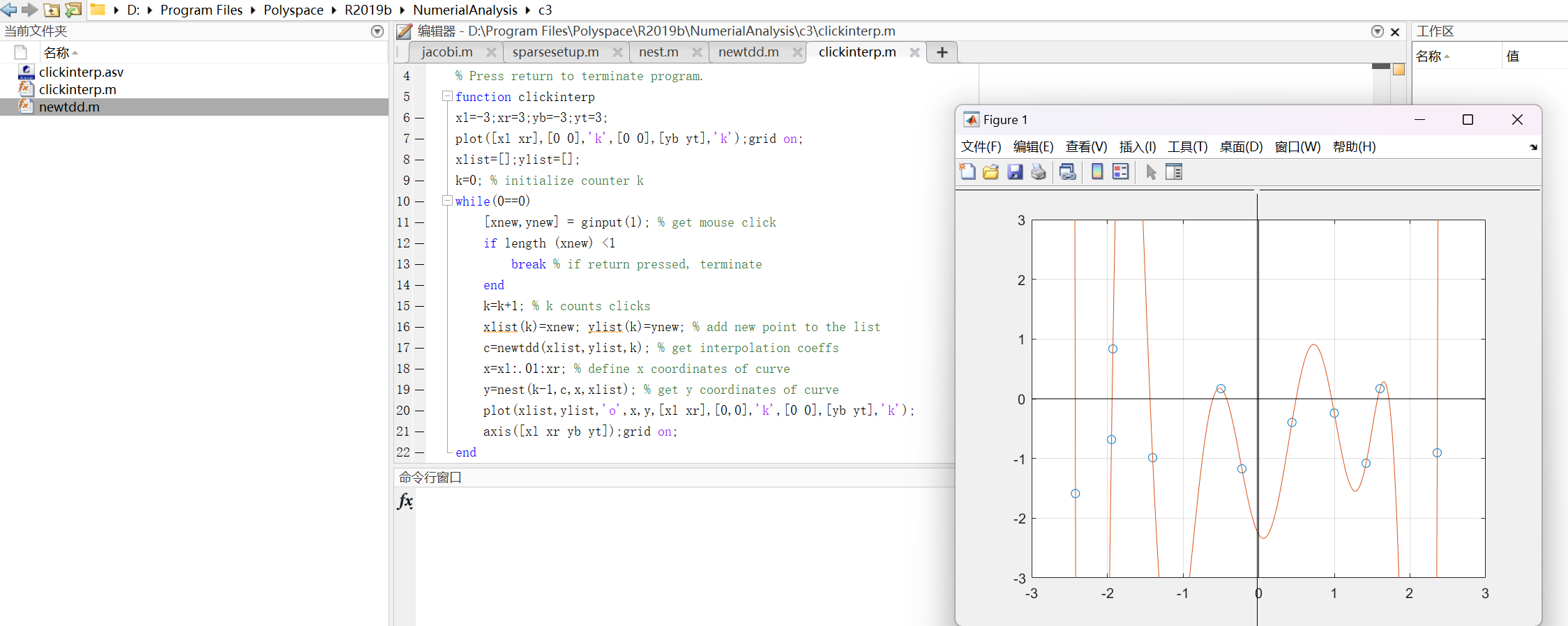
Note that nest.m is in Chapter0, so you can add this file to search path, the program will run successfully.

1
2
3
4
5
6
7
8
9
10
11
12
13
14
15
16
17
18
19
20
21
22
23

%clickinterp.m
%Program 3.2. Polynomial Interpolation Program
%Click in MATLAB figure window to locate data point.
% Continue, to add more points.
% Press return to terminate program.
function clickinterp
xl=-3;xr=3;yb=-3;yt=3;
plot([xl xr],[0 0],'k',[0 0],[yb yt],'k');grid on;
xlist=[];ylist=[];
k=0; % initialize counter k
while(0==0)
    [xnew,ynew] = ginput(1); % get mouse click
    if length (xnew) <1
        break % if return pressed, terminate
    end
    k=k+1; % k counts clicks
    xlist(k)=xnew; ylist(k)=ynew; % add new point to the list
    c=newtdd(xlist,ylist,k); % get interpolation coeffs
    x=xl:.01:xr; % define x coordinates of curve
    y=nest(k-1,c,x,xlist); % get y coordinates of curve
    plot(xlist,ylist,'o',x,y,[xl xr],[0,0],'k',[0 0],[yb yt],'k');
    axis([xl xr yb yt]);grid on;
end

Representing functions by approximating polynomials

💡For example💡:

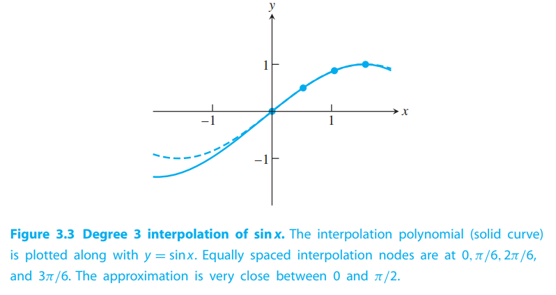
Interpolate the function $f(x) = \sin x$ at $4$ equally spaced points on $[0,\pi/2]$.

Solution:

The interval $[0,\pi/2]$ is a so-called fundamental domain for sine, meaning that an input from any other interval can be referred back to it.

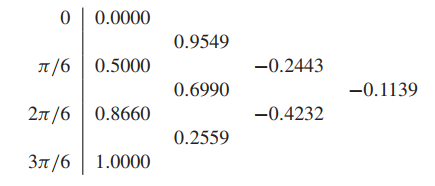
The degree 3 interpolating polynomial is therefore

$$
P_3(x) = 0 + x(0.9549 + (x − \pi/6)(−0.2443 + (x − \pi/3)(−0.1139)))
$$

1
2
3
4
5
6
7
8
9
10
11
12
13
14
15
16
17
18
19
20
21
22
23
24

%sin1.m
%Program 3.3 Building a sin calculator key, attempt #1
%Approximates sin curve with degree 3 polynomial
% (Caution: do not use to build bridges,
% at least until we have discussed accuracy.)
%Input: x
%Output: approximation for sin(x)
function y=sin1(x)
%First calculate the interpolating polynomial and
% store coefficients
b=pi*(0:3)/6;yb=sin(b); % b holds base points
c=newtdd(b,yb,4);
%For each input x, move x to the fundamental domain and evaluate
% the interpolating polynomial
s=1; % Correct the sign of sin
x1=mod(x,2*pi);
if x1>pi
    x1 = 2*pi-x1;
    s = -1;
end
if x1 > pi/2
    x1 = pi-x1;
end
y = s*nest(3,c,x1,b);

Interpolation Error

Interpolation error formula

THEOREM 3.4
Assume that $P(x)$ is the (degree $n − 1$ or less) interpolating polynomial fitting the $n$ points $(x_1,y_1), . . . , (x_n,y_n)$. The interpolation error is
$$
f(x) - P(x) = \frac{(x-x_1)(x-x_2)\cdots(x-x_n)}{n!}f^{(n)}(c)
\tag{3.6}
$$
where $c$ lies between the smallest and largest of the numbers $x,x_1, . . . , x_n$.

💡For example💡:
Still $f(x) = \sin x, x \in [0, \pi/2]$. Cal the 4 points interpolation error.

By (3.6), we get,
$$
\sin x - P(x) = \frac{(x-0)(x-\frac{\pi}{6})(x-\frac{\pi}{3})(x-\frac{\pi}{2})}{4!} f’’’’(c),
0 < c < \pi/2
$$

The fourth derivative $f’’’’(c) = \sin c$. At worst, $|\sin c|$ is no more than 1, so we can be assured of an upper bound on interpolation error:
$$
|\sin x - P(x)| \leq \frac{(x-0)(x-\frac{\pi}{6})(x-\frac{\pi}{3})(x-\frac{\pi}{2})}{24} |1|
$$

Note that the interpolation error will tend to be smaller close to the center of the interpolation interval.

Proof of Newton form and error formula

to be added…

Runge phenomenon（龙格现象）

For example:

Interpolate $f(x) = 1/(1 + 12x^2)$ at evenly spaced points in $[−1,1]$.

Runge phenomenon: polynomial wiggle near the ends of the interpolation interval.

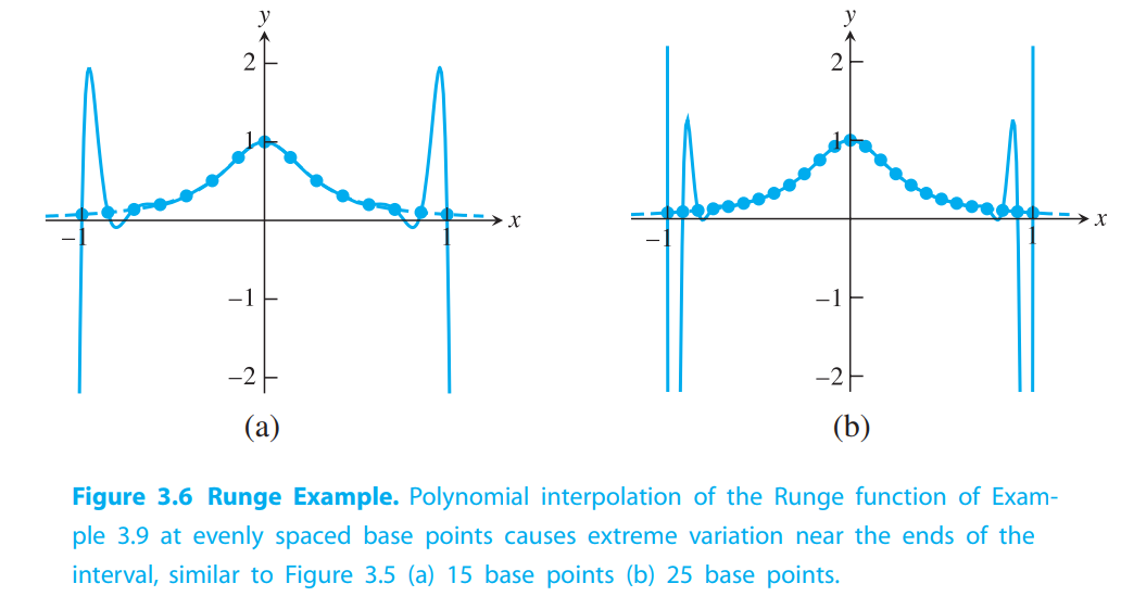
The cure for this problem is intuitive: Move some of the interpolation points toward the outside of the interval, where the function producing the data can be better fit.

Chebyshev Interpolation

It turns out that the choice of base point spacing can have a significant effect on the interpolation error. Chebyshev interpolation refers to a particular optimal way of spacing the points.

Chebyshev’s theorem

The interpolation error is
$$
\frac{(x-x_1)(x-x_2)\cdots(x-x_n)}{n!}f^{(n)}(c)
$$
Let’s fix the interval to be $[−1,1]$ for now.

The numerator of the interpolation error formula is itself a degree $n$ polynomial in $x$ and has some maximum value on $[−1,1]$.

$$
(x-x_1)(x-x_2)\cdots(x-x_n)
\tag{3.9}
$$

We need to minimum it. So this is called the minimax problem of interpolation.

THEOREM 3.6
The choice of real numbers $−1 \leq x_1, . . . , x_n \leq 1$ that makes the value of
$$
\underbrace{max}_{-1 \leq x \leq 1} |(x-x_1)(x-x_2)\cdots(x-x_n)|
$$
as small as possible is
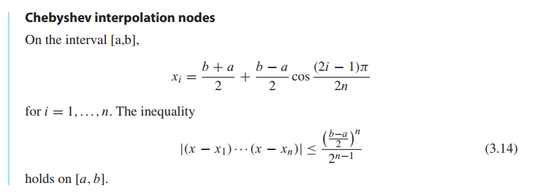
$$
x_i = \cos\frac{(2i-1)\pi}{2n}, for, i = 1, \cdots, n
$$
and the minimum value is $\frac{1}{2^{n-1}}$. In fact, the minimum is achieved by
$$
(x-x_1)(x-x_2)\cdots(x-x_n) = \frac{1}{2^{n-1}}T_n(x)
$$
where $T_n(x)$ denotes the degree $n$ Chebyshev polynomial（$n$阶切比雪夫多项式）.

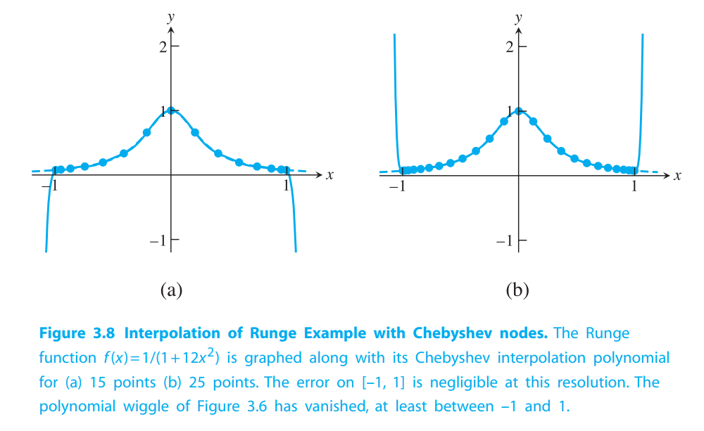
We conclude from the theorem that interpolation error can be minimized if the $n$ interpolation base points in $[−1,1]$ are chosen to be the roots of the degree $n$ Chebyshev polynomial $T_n(x)$.

We will call the interpolating polynomial that uses the Chebyshev roots as base points the Chebyshev interpolating polynomial（$n-1$阶切比雪夫插值多项式）.

Chebyshev polynomials

The $n$th Chebyshev polynomial is
$$
T_n(x) = \cos(n \arccos x)
$$
Set $y = \arccos x$, so that $\cos y = x$.

$$
T_{n+1}(x) = 2xT_n(x) - T_{n-1}(x)
\tag{3.13}
$$
is called the recursion relation for the Chebyshev polynomials. Several facts follow
from (3.13):

FACT 1
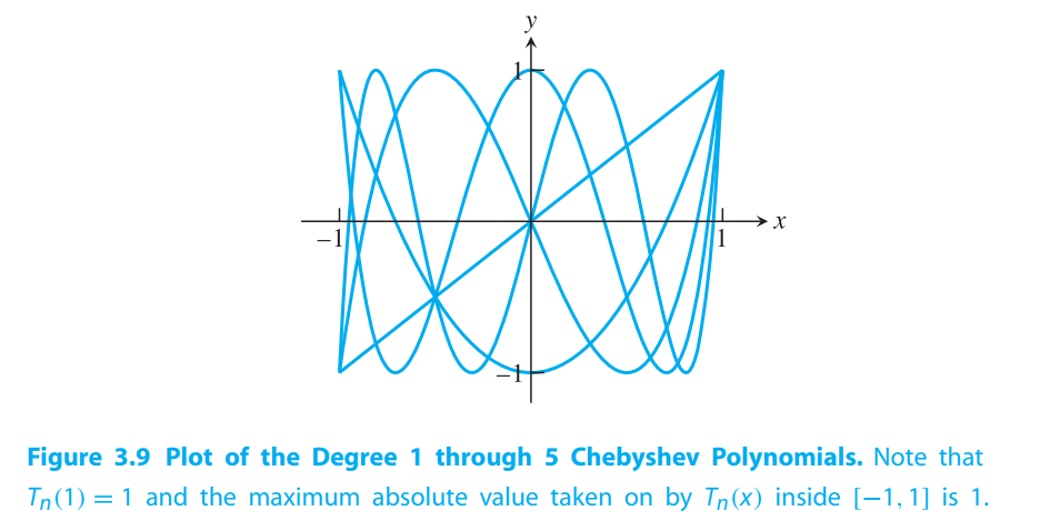
The $T_n$’s are polynomials. We showed this explicitly for $T_0,T_1, and T_2$. Since $T_3$ is a polynomial combination of $T_1$ and $T_2$, $T_3$ is also a polynomial. The same argument goes for all $T_n$. The first few Chebyshev polynomials (see Figure 3.9) are
$$
T_0(x) = 1\\
T_1(x) = x\\
T_2(x) = 2x^2-1\\
T_3(x) = 4x^3 - 3x\\
$$

FACT 2
$deg(T_n) = n$, and the leading coefficient is $2n−1$. This is clear for $n = 1$ and $2$, and the recursion relation extends the fact to all $n$.

FACT 3
$T_n(1) = 1$ and $T_n(−1) = (−1)^n$.

FACT 4
The maximum absolute value of $T_n(x)$ for $−1 \leq x \leq 1$ is $1$. This follows immediately from the fact that $T_n(x) = \cos y$ for some $y$.

FACT 5
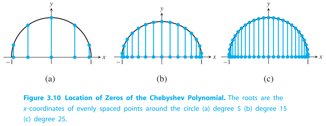
All zeros of $T_n(x)$ are located between $−1$ and $1$. See Figure 3.10. In fact, the zeros are the solution of $0 = cos(n \arccos x)$. Since $cosy = 0$ if and only if $y = odd-integer \cdot (\pi/2)$, we find that
$$
n\arccos x = odd \cdot \pi/2\\
x = \cos \frac{odd \cdot \pi}{2n}
$$

Change of interval

Cubic Splines

Properties of splines

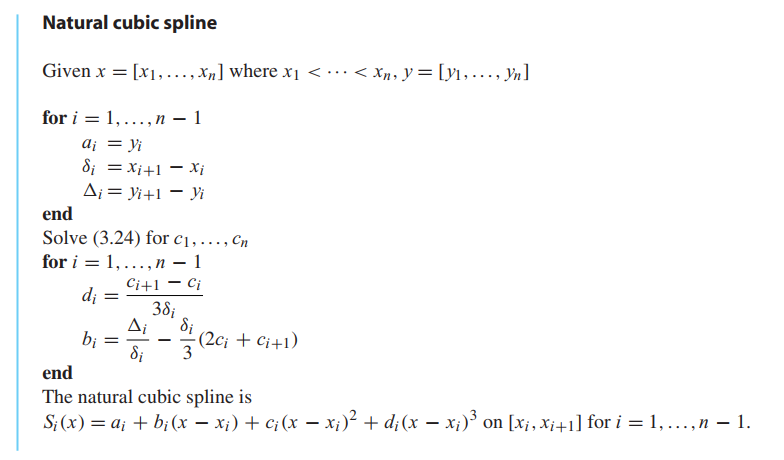
A cubic spline $S(x)$ through the data points $(x_1,y_1), . . . , (x_n,y_n)$ is a set of cubic polynomials

$$
S_1(x) = y_1 + b_1(x-x_1) + c_1(x-x_1)^2 + d_1(x - x_1)^3, on [x_1,x_2]\\
S_2(x) = y_2 + b_2(x-x_2) + c_2(x-x_2)^2 + d_2(x - x_2)^3, on [x_2,x_3]\\
\cdots\\
S_{n-1}(x) = y_{n-1} + b_{n-1}(x-x_{n-1}) + c_{n-1}(x-x_{n-1})^2 + d_{n-1}(x - x_{n-1})^3, on [x_{n-1},x_n]
\tag{3.17}
$$

with the following properties:

Property 1
$$
S_i(x_i) = y_i\\
S_i(x_{i+1}) = y_{i+1}, i = 1, \cdots, n-1
$$

Property 2
$$
S’_{i-1}(x_i) = S’_i(x_i), i = 2, \cdots, n-1, slope
$$

Property 3
$$
S’’_{i-1}(x_i) = S’’_i(x_i), i = 2, \cdots, n-1, curvature
$$

Property 4a Natural spline.
$$
S_1’’(x_1) = 0, S’’_{n-1}(x_n) = 0
$$

Constructing a spline from a set of data points means finding the coefficients $b_i,c_i,d_i$ that make Properties 1–3 hold.

THEOREM 3.7
Let $n \neq 2$. For a set of data points $(x_1,y_1), . . . , (x_n,y_n)$ with distinct $x_i$, there is a unique natural cubic spline fitting the points.

Endpoint conditions

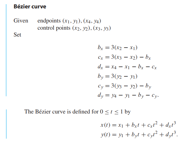
Bézier Curves

Reality Check 3: Fonts from Bézier curves