Keywords: Gaussian Distribution, The Exponential Family, Python
This is the Chapter2 ReadingNotes from book Bishop-Pattern-Recognition-and-Machine-Learning-2006. [Code_Python]
One role for the distributions discussed in this chapter is to model the probability distribution $p(\pmb{x})$ of a random variable $\pmb{x}$, given a finite set $\lbrace \pmb{x_1}, \cdots , \pmb{x_N} \rbrace$ of observations. This problem is known as density estimation.
Binary Variables
We begin by considering a single binary random variable $x \in \lbrace 0,1 \rbrace$. For example, $x$ might describe the outcome of flipping a coin, with $x = 1$ representing ‘heads’, and x = 0 representing ‘tails’.
The probability of $x = 1$ will be denoted by the parameter $\mu$ so that
$$
p(x=1|\mu) = \mu
\tag{2.1}
$$
where $0 \leq \mu \leq 1$, from which it follows that $p(x = 0|\mu) = 1 − \mu$. The probability distribution over $x$ can therefore be written in the form
$$
Bern(x | \mu) = \mu^x (1-\mu)^{1-x}
\tag{2.2}
$$
which is known as the Bernoulli distribution 伯努利分布.
It is easily verified that this distribution is normalized and that it has mean and variance given by
$$
E[x] = \mu
\tag{2.3}
$$
$$
var[x] = \mu(1-\mu)
\tag{2.4}
$$
Suppose we have a data set $D = \lbrace x_1, \cdots , x_N \rbrace$ of observed values of $x$, iid, so the likelyhood function is
$$
p(D|\mu) = \prod_{n=1}^{N} p(x_n|\mu) = \prod_{n=1}^{N} \mu^{x_n} (1 - \mu)^{1-x_n}
\tag{2.5}
$$
$$
\ln p(D|\mu) = \sum_{n=1}^{N} \ln p(x_n|\mu) = \sum_{n=1}^{N} \lbrace x_n\ln \mu + (1-x_n)\ln(1 - \mu) \rbrace
\tag{2.6}
$$
If we set the derivative of $\ln p(D|\mu)$ with respect to $\mu$ equal to zero, we obtain the maximum likelihood estimator
$$
\mu_{ML} = \frac{1}{N}\sum_{n=1}^{N} x_n
\tag{2.7}
$$
which is also known as the sample mean.
If we denote the number of observations of $x = 1$ (heads) within this data set by $m$, then we can write (2.7) in the form
$$
\mu_{ML} = \frac{m}{N}
\tag{2.8}
$$
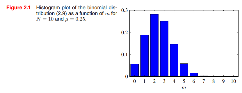
We can also work out the distribution of the number $m$ of observations of $x = 1$, given that the data set has size $N$. This is called the binomial distribution 二项分布,
$$
Bin(m|N,\mu) = \begin{pmatrix}
N\\m
\end{pmatrix} \mu^m (1-\mu)^{N-m}
\tag{2.9}
$$
$$
E[m] = \sum_{m=1}^N m Bin(m|N,\mu) = N\mu\tag{2.11}
$$
$$
var[m] = N\mu(1-\mu)
\tag{2.12}
$$
The beta distribution
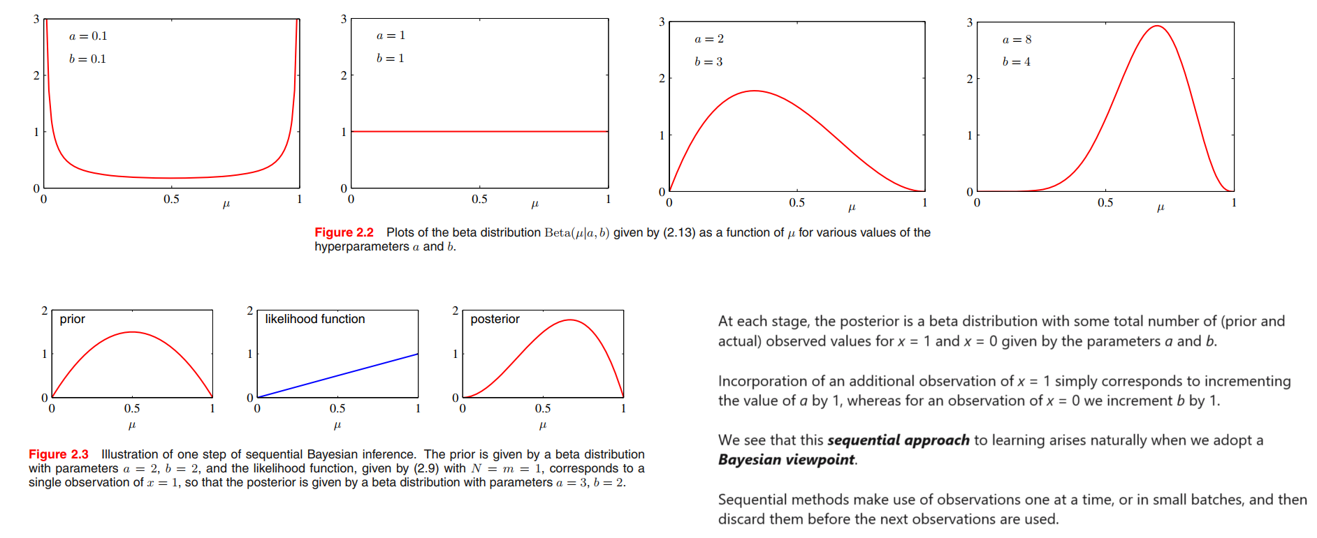
we note that the likelihood function takes the form of the product of factors of the form $\mu^{x} (1 - \mu)^{1-x}$.
If we choose a prior to be proportional to powers of $\mu$ and $(1 − \mu)$, then the posterior distribution, which is proportional to the product of the prior and the likelihood function, will have the same functional form as the prior. This property is called conjugacy 共轭.
We therefore choose a prior, called the beta distribution, given by
$$
Beta(\mu | a, b) = \frac{\Gamma (a+b)}{\Gamma(a) \Gamma(b)} \mu^{a-1}(1-\mu)^{b-1}
\tag{2.13}
$$
where $\Gamma(x)$ is the gamma function defined as
$$
\Gamma(t) = \int_0^{+\infty} x^{t-1}e^{-x}dx, t>0
$$
$$
\int_0^1 Beta(\mu | a, b) d\mu = 1
\tag{2.14}
$$
The mean and variance of the beta distribution are given by
$$
E[\mu] = \frac{a}{a+b}
\tag{2.15}
$$
$$
var[\mu] = \frac{ab}{(a+b)^2 (a+b+1)}
\tag{2.16}
$$
By Bayes’s Therom and (2.13) and (2.9), this posterior distribution
$$
p(\mu|m,l,a,b) \propto \mu^{m+a-1}(1-\mu)^{l+b-1}, l = N-m
\tag{2.17}
$$
it is simply another beta distribution, and its normalization coefficient can therefore be obtained by comparison with (2.13) to give
$$
p(\mu|m,l,a,b) = \frac{\Gamma (m+a+l+b)}{\Gamma(m+a) \Gamma(l+b)} \mu^{m+a-1}(1-\mu)^{l+b-1}, l = N-m
\tag{2.18}
$$

we must evaluate the predictive distribution of $x$, given the observed data set $D$.
$$
\begin{aligned}
p(x=1|D) &= \int_0^1 p(x=1|\mu)p(\mu|D) d\mu \\ &= \int_0^1 \mu p(\mu|D)d\mu \\ &= E[\mu|D]\\
\underset{Together with (2.18),(2.15)}{\longrightarrow}
&= \frac{m+a}{m+a+l+b}
\end{aligned}
\tag{2.19}
$$
贝叶斯视角下的后验概率的均值,随着观察数据的增多,越来越趋向于最大似然数得到的结果。
Multinomial Variables
If we have a variable that can take $K = 6$ states and a particular observation of the variable happens to correspond to the state where $x_3 = 1$, then $\pmb{x}$ will be represented by
$$
\pmb{x} = (0,0,1,0,0,0)^T
$$
where, $\sum_{k=1}^{K} x_k = 1$.
If we denote the probability of $x_k = 1$ by the parameter $\mu_k$, then the distribution of $\pmb{x}$ is given
$$
p(\pmb{x}|\pmb{\mu}) = \prod_{k=1}^{K} \mu_k^{x_k}
\tag{2.26}
$$
where, $\pmb{\mu} = (\mu_1, \cdots, \mu_K)^T$ and, $\sum_{k} \mu_k = 1$
The distribution (2.26) can be regarded as a generalization of the Bernoulli distribution to more than two outcomes. It is easily seen that the distribution is normalized
$$
\sum_{\pmb{x}} p(\pmb{x}|\pmb{\mu}) = \sum_{k=1}^{K} \mu_k = 1
$$
and
$$
E[\pmb{x}|\pmb{\mu}] = \sum_{\pmb{x}} p(\pmb{x}|\pmb{\mu}) \pmb{x} = \pmb{\mu}
\tag{2.28}
$$
By maximum likelihood, we get
$$
\mu_k^{ML} = \frac{m_k}{N}
\tag{2.33}
$$
which is the fraction of the $N$ observations for which $x_k = 1$.
The multinomial distribution is:
$$
Mult(m_1, m_2, \cdots, m_K | \pmb{\mu}, N) = \begin{pmatrix}N \\ m_1m_2\cdots m_K\end{pmatrix}\prod_{k=1}^{K} \mu_k^{m_k}
\tag{2.34}
$$
The Dirichlet distribution
By inspection of the form of the multinomial distribution, we see that the conjugate prior is given by
$$
p(\pmb{\mu}|\pmb{\alpha}) \propto \prod_{k=1}^{K} \mu_k ^{\alpha_{k}-1}
$$
the Dirichlet distribution is:
$$
Dir(\pmb{\mu}|\pmb{\alpha}) = \frac{\Gamma{(\alpha_0)}}{\Gamma{(\alpha_1)} \cdots \Gamma{(\alpha_K)}} \prod_{k=1}^K \mu_k^{\alpha_k - 1}
\tag{2.38}
$$
Multiplying the prior (2.38) by the likelihood function (2.34), we obtain the posterior distribution for the parameters ${\mu_k}$ in the form
$$
p(\pmb{\mu}|D,\pmb{alpha}) \propto p(D|\pmb{\mu}) p(\pmb{\mu}|\pmb{alpha}) \propto \prod_{k=1}^{K} \mu_k^{\alpha_k + m_k - 1}
\tag{2.40}
$$
We see that the posterior distribution again takes the form of a Dirichlet distribution, confirming that the Dirichlet is indeed a conjugate prior for the multinomial.

The Gaussian Distribution
For a $D$-dimensional vector $\pmb{x}$, the multivariate Gaussian distribution takes the form
$$
\mathcal{N}(\pmb{x} | \pmb{\mu}, \pmb{\Sigma}) = \frac{1}{(2\pi)^{D/2}}\frac{1}{|\pmb{\Sigma}|^{1/2}} exp \lbrace -\frac{1}{2}(\pmb{x - \mu})^T \pmb{\Sigma}^{-1}(\pmb{x-\mu}) \rbrace
\tag{2.43}
$$
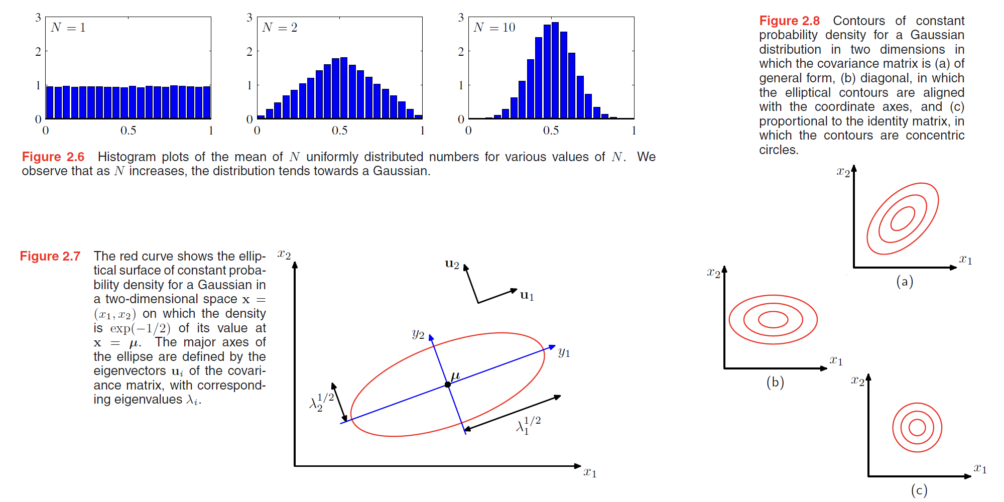
Gaussian distribution arises is when we consider the sum of multiple random variables. The central limit theorem (due to Laplace) tells us that, subject to certain mild conditions, the sum of a set of random variables, which is of course itself a random variable, has a distribution that becomes increasingly Gaussian as the number of terms in the sum increases (Walker, 1969).
We begin by considering the geometrical form of the Gaussian distribution. The functional dependence of the Gaussian on $x$ is through the quadratic form (高斯函数对$x$的函数依赖性通过二次形式表现)
$$
\Delta^2 = (\pmb{x - \mu})^T \Sigma^{-1} (\pmb{x - \mu})
\tag{2.44}
$$
The quantity $\Delta$ is called the Mahalanobis distance from $\pmb{\mu}$ to $\pmb{x}$ and reduces to the Euclidean distance when $\Sigma$ is the identity matrix. The Gaussian distribution will be constant on surfaces in x-space for which this quadratic form is constant.
The covariance matrix $\Sigma$ is a symmetric matrix, it can be expressed as an expansion in terms of its eigenvectors in the form
$$
\Sigma = \sum_{i=1}^{D} \lambda_i \pmb{u_i u_i^T}
\tag{2.48}
$$
👉More about Symmetric matrix and EigenVectors >>
$$
\Sigma^{-1} = \sum_{i=1}^{D} \frac{1}{\lambda_i} \pmb{u_i u_i^T}
\tag{2.49}
$$
Substituting (2.49) into (2.44), the quadratic form becomes
$$
\Delta^2 = \sum_{i=1}^{D} \frac{y_i^2}{\lambda_i}
\tag{2.50}
$$
where we have defined
$$
y_i = \pmb{u_i}^T(\pmb{x-\mu})
\tag{2.51}
$$
$\pmb{x^TAx} = \pmb{y^TDy}$ where, $\pmb{x = Py}$ and $\pmb{P}$ is a matrix of eigen vectors of $\pmb{A}$.
We can interpret ${y_i}$ as a new coordinate system defined by the orthonormal vectors $\pmb{u_i}$ that are shifted and rotated with respect to the original $x_i$ coordinates. Forming the vector $\pmb{y} = (y_1, \cdots, y_D)^T$, we have
$$
\pmb{y = U(x-\mu)}
\tag{2.52}
$$
The quadratic form, and hence the Gaussian density, will be constant on surfaces for which (2.51) is constant.
Now consider the form of the Gaussian distribution in the new coordinate system defined by the $y_i$.
In going from the $\pmb{x}$ to the $\pmb{y}$ coordinate system, we have a Jacobian matrix $J$ with elements given by
$$
J_{ij} = \frac{\partial x_i}{\partial y_j} = U_{ji}
\tag{2.53}
$$
thus
$$
|J|^2 = |U^T|^2 = 1
\tag{2.54}
$$
the determinant $|\Sigma|$ of the covariance matrix can be written as the product of its eigenvalues, and hence
$$
|\Sigma|^{1/2} = \prod_{j=1}^{D}\lambda_j^{1/2}
\tag{2.55}
$$
Thus in the $y_j$ coordinate system, the Gaussian distribution takes the form
$$
p(\pmb{y}) = p(\pmb{x})|J| = \prod_{j=1}^{D} \frac{1}{(2\pi\lambda_j)^{1/2}} exp\lbrace -\frac{y_j^2}{2\lambda_j} \rbrace
\tag{2.56}
$$
which is the product of $D$ independent univariate Gaussian distributions. ($D$ is the dimension of the vector, like $D = 2$, $\pmb{x} = (x_1, x_2)$)
The eigenvectors therefore define a new set of shifted and rotated coordinates with respect to which the joint probability distribution factorizes into a product of independent distributions. The integral of the distribution in the $\pmb{y}$ coordinate system is then
$$
\int p(\pmb{y}) d\pmb{y} = \prod_{j=1}^{D} \int_{-\infty}^{\infty} \frac{1}{(2\pi\lambda_j)^{1/2}} exp\lbrace -\frac{y_j^2}{2\lambda_j} \rbrace dy_j = 1
\tag{2.57}
$$
where we have used the result (1.48) for the normalization of the univariate Gaussian. This confirms that the multivariate Gaussian (2.43) is indeed normalized.
$$
\int_{-\infty}^{\infty} \mathcal{N}(x|\mu, \sigma^2) dx = 1
\tag{1.48}
$$
We now look at the moments of the Gaussian distribution and thereby provide an interpretation of the parameters $\pmb{\mu}$ and $\Sigma$.
https://en.wikipedia.org/wiki/Moment_(mathematics)
The expectation of $\pmb{x}$ under the Gaussian distribution is given by
$$
\begin{aligned}
E[\pmb{x}] &= \frac{1}{(2\pi)^{D/2}}\frac{1}{|\pmb{\Sigma}|^{1/2}} \int exp \lbrace -\frac{1}{2}(\pmb{x - \mu})^T \pmb{\Sigma}^{-1}(\pmb{x-\mu}) \rbrace \pmb{x} d\pmb{x}\\
&= \frac{1}{(2\pi)^{D/2}}\frac{1}{|\pmb{\Sigma}|^{1/2}} \int exp \lbrace -\frac{1}{2}\pmb{z}^T \pmb{\Sigma}^{-1}\pmb{z} \rbrace (\pmb{z+\mu}) d\pmb{z}\\
&= \pmb{\mu}
\end{aligned}
\tag{2.58}
$$
and so we refer to $\pmb{\mu}$ as the mean of the Gaussian distribution.
We now consider second order moments of the Gaussian.(variance)
In the univariate case,
$$
E[x^2] = \int_{-\infty}^{\infty} N(x|\mu, \sigma^2) x^2 dx = \mu^2 + \sigma^2
\tag{1.50}
$$
$$
var[x] = E[x^2] - E[x]^2 = \sigma^2
\tag{1.51}
$$
thus, For the multivariate Gaussian
$$
\begin{aligned}
E[\pmb{xx^T}] &= \frac{1}{(2\pi)^{D/2}}\frac{1}{|\pmb{\Sigma}|^{1/2}} \int exp \lbrace -\frac{1}{2}(\pmb{x - \mu})^T \pmb{\Sigma}^{-1}(\pmb{x-\mu}) \rbrace \pmb{xx^T} d\pmb{x}\\
&= \frac{1}{(2\pi)^{D/2}}\frac{1}{|\pmb{\Sigma}|^{1/2}} \int exp \lbrace -\frac{1}{2}\pmb{z}^T \pmb{\Sigma}^{-1}\pmb{z} \rbrace (\pmb{z+\mu})(\pmb{z+\mu})^T d\pmb{z}\\
&= \pmb{\mu\mu^T} + \frac{1}{(2\pi)^{D/2}}\frac{1}{|\pmb{\Sigma}|^{1/2}} \int exp \lbrace -\frac{1}{2}\pmb{z}^T \pmb{\Sigma}^{-1}\pmb{z} \rbrace \pmb{z}\pmb{z}^T d\pmb{z}\\
&= \pmb{\mu\mu^T} + \sum_{i=1}^{D} \pmb{u_iu_i^T}\lambda_i\\
&= \pmb{\mu\mu^T} + \Sigma
\end{aligned}
\tag{2.61}
$$
where,
$$
\begin{aligned}
\pmb{z} &= \pmb{x-\mu}\\
&= \sum_{j=1}^{D} y_j \pmb{u_j}
\end{aligned}
\tag{2.60}
$$
thus,
$$
cov[\pmb{x}] = \Sigma
\tag{2.64}
$$

Gaussian distribution has some sever limitations:
- to many parameters, computation expensive.
- intrinsically unimodal(单峰), unable to provide a good approximation to multimodal distributions.
We will see later that the introduction of latent variables, also called hidden variables or unobserved variables, allows both of these problems to be addressed.
Conditional Gaussian distributions
Suppose $\pmb{x}$ is a $D$-dimensional vector with Gaussian distribution $N(\pmb{x}|\pmb{\mu}, \Sigma)$ and that we partition $\pmb{x}$ into two disjoint subsets $\pmb{x}_a$ and $\pmb{x}_b$. Without loss of generality, we can take $\pmb{x}_a$ to form the first $M$ components of $\pmb{x}$, with $\pmb{x}_b$ comprising the remaining $D−M$ components, so that
$$
\pmb{x} = \begin{pmatrix} \pmb{x_a} \\ \pmb{x_b}\end{pmatrix}
\tag{2.65}
$$
corresponding partitions of the mean vector $\pmb{\mu}$ and covariance matrix $\Sigma$ given by
$$
\pmb{\mu} = \begin{pmatrix} \pmb{\mu_a} \\ \pmb{\mu_b}\end{pmatrix}
\tag{2.66}
$$
$$
\Sigma = \begin{bmatrix} \Sigma_{aa} & \Sigma_{ab} \\ \Sigma_{ba} & \Sigma_{bb}\end{bmatrix}
\tag{2.67}
$$
where, $\Sigma^T = \Sigma$. The precision matrix $\Lambda = \Sigma^{-1}$.
Conditional distribution $p(\pmb{x_a|x_b})$ will be Gaussian:
$$
\pmb{\mu_{a|b}} = \pmb{\mu_a} + \Sigma_{ab}\Sigma_{bb}^{-1}(\pmb{x_b}-\pmb{\mu_b})
\tag{2.81}
$$
$$
\Sigma_{a|b} = \Sigma_{aa} - \Sigma_{ab}\Sigma_{bb}^{-1}\Sigma_{ba}
\tag{2.82}
$$
Note that the mean of the conditional distribution $p(\pmb{x_a|x_b})$, given by (2.81), is a linear function of $\pmb{x_b}$ and that the covariance, given by (2.82), is independent of $\pmb{x_a}$. This represents an example of a linear-Gaussian model.
Marginal Gaussian distributions
Now we turn to a discussion of the marginal distribution given by
$$
p(\pmb{x_a}) = \int p(\pmb{x_a, x_b}) d\pmb{x_b}
\tag{2.83}
$$
which, as we shall see, is also Gaussian.

Bayes’ theorem for Gaussian variables
Here we shall suppose that we are given a Gaussian marginal distribution $p(\pmb{x})$ and a Gaussian conditional distribution $p(\pmb{y}|\pmb{x})$ in which $p(\pmb{y}|\pmb{x})$ has a mean that is a linear function of $\pmb{x}$, and a covariance which is independent of $\pmb{x}$.

Maximum likelihood for the Gaussian
Given a data set $\pmb{X} = (\pmb{x_1}, \cdots , \pmb{x_N})^T$ in which the observations $\lbrace \pmb{x_n} \rbrace$ are assumed to be drawn independently from a multivariate Gaussian distribution, we can estimate the parameters of the distribution by maximum likelihood, and get
$$
\pmb{\mu_{ML}} = \frac{1}{N} \sum_{n=1}^{N}\pmb{x_n}
$$
$$
\pmb{\widetilde{\Sigma}} = \frac{1}{N-1} \sum_{n=1}^{N}(\pmb{x_n}-\pmb{\mu_{ML}})(\pmb{x_n}-\pmb{\mu_{ML}})^T
$$
Sequential estimation
Sequential methods allow data points to be processed one at a time and then discarded and are important for on-line applications, and also where large data sets are involved so that batch processing of all data points at once is infeasible.
Bayesian inference for the Gaussian
The maximum likelihood framework gave point estimates for the parameters $\pmb{\mu}$ and $\pmb{\Sigma}$. Now we develop a Bayesian treatment by introducing prior distributions over these parameters.
We shall suppose that the variance $\sigma^2$ is known, and we consider the task of inferring the mean $\mu$ given a set of $N$ observations $\pmb{X} = \lbrace x_1, \cdots , x_N \rbrace $. The likelihood function, that is the probability of the observed data given $\mu$, viewed as a function of $\mu$, is given by
$$
\begin{aligned}
p(\pmb{X}|\mu) &= \prod_{n=1}^{N} p(x_n|\mu) \\
&= \frac{1}{(2\pi\sigma^2)^{N/2}} exp \lbrace -\frac{1}{2\sigma^2} \sum_{n=1}^{N} (x_n - \mu)^2\rbrace
\end{aligned}
\tag{2.137}
$$
the posterior distribution is given by,
$$
p(\mu|\pmb{X}) \propto p(\pmb{X}|\mu)p(\mu)
\tag{2.139}
$$
where
$$
p(\mu) = N(\mu|mu_0, \sigma_0^2)
\tag{2.138}
$$
thus, we get
$$
\mu_N = \frac{\sigma^2}{N\sigma_0^2 + \sigma^2}\mu_0 + \frac{N\sigma_0^2}{N\sigma_0^2+\sigma^2}\mu_{ML}
\tag{2.141}
$$
$$
\frac{1}{\sigma_N^2} = \frac{1}{\sigma_0^2} + \frac{N}{\sigma^2}
\tag{2.142}
$$
In fact, the Bayesian paradigm leads very naturally to a sequential view of the inference problem. To see this in the context of the inference of the mean of a Gaussian, we write the posterior distribution with the contribution from the final data point $\pmb{x_N}$ separated out so that
$$
p(\pmb{\mu}|D) \propto [ p(\pmb{\mu}) \prod_{n=1}^{N-1} p(\pmb{x_n}|\pmb{\mu}) ] p(\pmb{x_N}|\pmb{\mu})
$$
The term in square brackets is (up to a normalization coefficient) just the posterior distribution after observing $N − 1$ data points. We see that this can be viewed as a prior distribution, which is combined using Bayes’ theorem with the likelihood function associated with data point $\pmb{x_N}$ to arrive at the posterior distribution after observing $N$ data points. This sequential view of Bayesian inference is very general and applies to any problem in which the observed data are assumed to be independent and identically distributed.
So far, we have assumed that the variance of the Gaussian distribution over the data is known and our goal is to infer the mean. Now let us suppose that the mean is known and we wish to infer the variance.
Let $\lambda \equiv \frac{1}{\sigma^2}$, then,
$$
\begin{aligned}
p(\pmb{X}|\lambda) &= \prod_{n=1}^{N} N(x_n | \mu, \lambda^{-1}) \\
&\propto \lambda^{N/2} exp \lbrace -\frac{\lambda}{2} \sum_{n=1}^{N} (x_n - \mu)^2\rbrace
\end{aligned}
\tag{2.145}
$$
the posterior distribution we get is
$$
p(\lambda|\pmb{X}) \propto \lambda^{a_0 - 1} \lambda^{N/2} exp \lbrace -b_0\lambda - \frac{\lambda}{2} \sum_{n=1}^{N} (x_n - \mu)^2 \rbrace
\tag{2.149}
$$
where the prior distribution of $\lambda$ is
$$
Gam(\lambda|a,b) = \frac{1}{\Gamma(a)} b^a \lambda^{a-1} exp(-b\lambda)
\tag{2.146}
$$
we get
$$
a_N = a_0 + \frac{N}{2}
\tag{2.150}
$$
$$
b_N = b_0 + \frac{1}{2} \sum_{n=1}^{N} (x_n - \mu)^2 = b_0 + \frac{N}{2} \sigma^2_{ML}
\tag{2.151}
$$

Student’s t-distribution
If we have a univariate Gaussian $N(x|\mu, \tau)$ together with a Gamma prior $Gam(\tau | a, b)$ and we integrate out the precision, we obtain the marginal distribution of $x$ in the form
$$
\begin{aligned}
p(x | \mu, a, b) &= \int_0^\infty N(x | \mu, \tau^{-1}) Gam(\tau | a, b) d\tau \\
&= \frac{b^a}{\Gamma(a)} (\frac{1}{2\pi})^{1/2} [b+\frac{(x-\mu)^2}{2}]^{-a-1/2} \Gamma(a+1/2)
\end{aligned}
\tag{2.158}
$$
By convention we define new parameters given by $ν = 2a$ and $\lambda = a / b$, in terms of which the distribution $p(x|\mu, a, b)$ takes the form
$$
St(x|\mu, \lambda, v) = \frac{\Gamma (v / 2 + 1 / 2)}{\Gamma (v/2)} (\frac{\lambda}{\pi v})^{1/2} [1 + \frac{\lambda (x - \mu)^2}{v}]^{-v/2-1/2}
\tag{2.159}
$$
which is known as Student’s t-distribution. The parameter $\lambda$ is sometimes called the precision of the t-distribution, even though it is not in general equal to the inverse of the variance. The parameter $v$ is called the degrees of freedom, and its effect is illustrated in Figure 2.15.
From (2.158), we see that Student’s t-distribution is obtained by adding up an infinite number of Gaussian distributions having the same mean but different precisions.This gives the tdistribution an important property called robustness, which means that it is much less sensitive than the Gaussian to the presence of a few data points which are outliers. The robustness of the t-distribution is illustrated in Figure 2.16, which compares the maximum likelihood solutions for a Gaussian and a t-distribution

$$
St(\pmb{x}|\pmb{\mu, \Lambda}, v) = \frac{\Gamma(D/2+v/2)}{\Gamma(v/2)} \frac{|\Lambda|^{1/2}}{(\pi v)^{D/2}} [1+\frac{\Delta^2}{v}]^{-D/2-v/2}
\tag{2.162}
$$
where
$$
\Delta^2 = (\pmb{x-\mu}^T)\Lambda(\pmb{x-\mu})
\tag{2.163}
$$
This is the multivariate form of Student’s t-distribution and satisfies the following properties
$$
E[\pmb{x}] = \pmb{\mu}, v > 1\\
cov[\pmb{x}] = \frac{v}{(v-2)}\Lambda^{-1}, v > 2\\
mode[\pmb{x}] = \pmb{\mu}
$$
Periodic variables
Mixtures of Gaussians
We therefore consider a superposition of K Gaussian densities of the form
$$
p(\pmb{x}) = \sum_{k=1}^{K} \pi_k N(\pmb{x}|\pmb{\mu_K, \Sigma_k})
\tag{2.188}
$$
where
$$
\sum_{k=1}^K \pi_k = 1
\tag{2.189}
$$
which is called a mixture of Gaussians.

From the sum and product rules, the marginal density is given by
$$
p(\pmb{x}) = \sum_{k=1}^{K} p(k) p(\pmb{x}|k)
\tag{2.191}
$$
we can view $\pi_k = p(k)$ as the prior probability of picking the $k^{th}$ component, and the density $N(\pmb{x}|\pmb{\mu_k}, \Sigma_k) = p(\pmb{x}|k)$ as the probability of $\pmb{x}$ conditioned on $k$.
An important role is played by the posterior probabilities $p(k|\pmb{x})$, which are also known as responsibilities. From Bayes’ theorem it is given by
$$
\begin{aligned}
\gamma_k(\pmb{x}) &\equiv p(k|\pmb{x}) \\
&= \frac{p(k)p(\pmb{x}|k)}{\sum_l p(l)p(\pmb{x}|l)}\\
&= \frac{\pi_k N(\pmb{x}|\pmb{\mu_k}, \Sigma_k)}{\sum_l \pi_l N(\pmb{x}|\pmb{\mu_l}, \Sigma_l)}
\end{aligned}
\tag{2.192}
$$
As a result, the maximum likelihood solution for the parameters no longer has a closed-form analytical solution. Alternatively we can employ a powerful framework called expectation maximization,
The Exponential Family
The exponential family of distributions over $\pmb{x}$, given parameters $\eta$, is defined to be the set of distributions of the form
$$
p(\pmb{x}|\pmb{\eta}) = h(\pmb{x})g(\pmb{\eta}) exp \lbrace \pmb{\eta^T} u(\pmb{x}) \rbrace
\tag{2.194}
$$
Here $\pmb{\eta}$ are called the natural parameters of the distribution, and $u(\pmb{x})$ is some function of $\pmb{x}$. The function $g(\pmb{\eta})$ can be interpreted as the coefficient that ensures that the distribution is normalized and therefore satisfies
$$
g(\pmb{\eta}) \int h(\pmb{x}) exp \lbrace \pmb{\eta^T} u(\pmb{x}) \rbrace d\pmb{x} = 1
\tag{2.159}
$$
Maximum likelihood and sufficient statistics
Taking the gradient of both sides of (2.195) with respect to $\pmb{\eta}$, we have
$$
\nabla g(\pmb{\eta}) \int h(\pmb{x}) exp \lbrace \pmb{\eta}^T u(\pmb{x}) \rbrace d\pmb{x} + g(\pmb{\eta}) \int h(\pmb{x}) exp \lbrace \pmb{\eta}^T u(\pmb{x}) \rbrace u(\pmb{x}) d\pmb{x} = 0
\tag{2.224}
$$
thus, we get
$$
-\nabla \ln g(\pmb{\eta}) = E[u(\pmb{x})]
\tag{2.226}
$$
Now consider a set of independent identically distributed data denoted by $\pmb{X} = \lbrace \pmb{x_1}, \cdots, \pmb{x_n} \rbrace$, for which the likelihood function is given by
$$
p(\pmb{X}|\pmb{\eta}) = (\prod_{n=1}^{N} h(\pmb{x_n})) g(\pmb{\eta})^N exp \lbrace \pmb{\eta}^T \sum_{n=1}^{N} u(\pmb{x_n})\rbrace
$$
Setting the gradient of $\ln p(\pmb{X}|\pmb{\eta})$ with respect to $\pmb{\eta}$ to zero, we get the following condition to be satisfied by the maximum likelihood estimator $\pmb{\eta}_{ML}$
$$
-\nabla \ln g(\pmb{\eta_{ML}}) = \frac{1}{N} \sum_{n=1}^{N} u(\pmb{x_n})
\tag{2.228}
$$
We see that the solution for the maximum likelihood estimator depends on the data only through $\sum_n u(\pmb{x_n})$, which is therefore called the sufficient statistic of the distribution (2.194). We do not need to store the entire data set itself but only the value of the sufficient statistic.
For the Bernoulli distribution, for example, the function $u(\pmb{x})$ is given just by $\pmb{x}$ and so we need only keep the sum of the data points $\lbrace \pmb{x_n} \rbrace $, whereas for the Gaussian $u(\pmb{x}) = (\pmb{x}, \pmb{x^2})^T$, and so we should keep both the sum of $\lbrace \pmb{x_n} \rbrace $ and the sum of $\lbrace \pmb{x_n^2} \rbrace $.
If we consider the limit $N \rightarrow \infty$, then the right-hand side of (2.228) becomes $E[u(\pmb{x})]$, and so by comparing with (2.226) we see that in this limit $\pmb{\eta_{ML}}$ will equal the true value $\pmb{\eta}$.
Conjugate priors
For any member of the exponential family (2.194), there exists a conjugate prior that can be written in the form
$$
p(\pmb{\eta}|\pmb{\chi}, v) = f(\pmb{\chi}, v) g(\pmb{\eta})^v exp \lbrace v \pmb{\eta}^T \pmb{\chi} \rbrace
\tag{2.229}
$$
the posterior distribution is like
$$
p(\pmb{\eta}|\pmb{X}, \pmb{\chi}, v) \propto g(\pmb{\eta})^{v+N} exp \lbrace \pmb{\eta}^T (\sum_{n=1}^N u(\pmb{x_n}) + v\pmb{\chi})\rbrace
$$
Noninformative priors
Nonparametric Methods
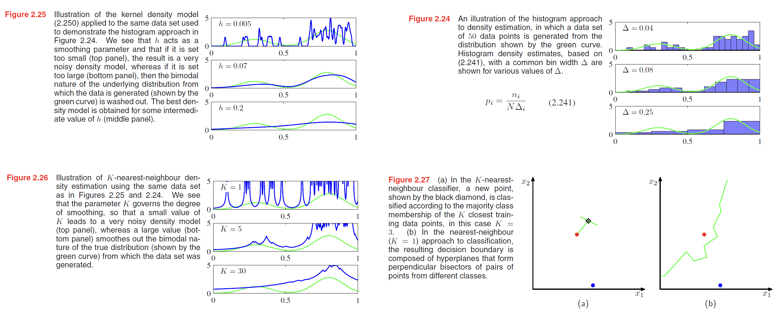
Throughout this chapter, we have focussed on the use of probability distributions having specific functional forms governed by a small number of parameters whose values are to be determined from a data set. This is called the parametric approach to density modelling.
An important limitation of this approach is that the chosen density might be a poor model of the distribution that generates the data, which can result in poor predictive performance. For instance, if the process that generates the data is multimodal, then this aspect of the distribution can never be captured by a Gaussian, which is necessarily unimodal.
we turn now to a discussion of two widely used nonparametric techniques for density estimation, kernel estimators and nearest neighbours.
Kernel density estimators
kernel density estimators:
$$
p(\pmb{x}) = \frac{1}{N} \sum_{n=1}^N \frac{1}{h^D} k(\frac{\pmb{x} - \pmb{x_n}}{h})
\tag{2.249}
$$
We can obtain a smoother density model if we choose a smoother kernel function, and a common choice is the Gaussian, which gives rise to the following kernel density model
$$
p(\pmb{x}) = \frac{1}{N} \sum_{n=1}^N \frac{1}{(2\pi h^2)^{1/2}} exp \lbrace -\frac{||\pmb{x}-\pmb{x_n}||^2}{2h^2} \rbrace
\tag{2.250}
$$


