Keywords: Camera calibration, motion Retargeting, python
This is the Chapter6 ReadingNotes from book Computer Animation_ Algorithms and Techniques_ Parent-Elsevier (2012).
Creating physically realistic motion using techniques involving key frames, forward kinematics, or inverse kinematics is a daunting task. In the previous chapters, techniques to move articulated linkages are covered, but they still require a large amount of animator talent in order to make an object move as in the real world.
Motion capture technologies
Electromagnetic tracking, also simply called magnetic tracking, uses sensors placed at the joints that transmit their positions and orientations back to a central processor to record their movements.
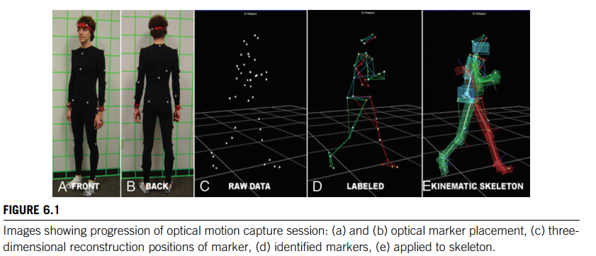
Optical markers, on the other hand, have a much larger range, and the performers only have to wear reflective markers on their clothes (see Figure 6.1, Color Plate 2).
Processing the images
The objective of motion control is to reconstruct the three-dimensional motion of a physical object and apply it to a synthetic model.
First, the two-dimensional images need to be processed so that the markers can be located, identified, and correlated in the multiple video streams.
Second, the three-dimensional locations of the markers need to be reconstructed from their two-dimensional locations.
Third, the three-dimensional marker locations must be constrained to a model of the physical system whose motion is being captured (e.g., a triangulated surface model of the performer).
The difference between the position of the marker and that of the joint is one source of error in motion capture systems.
Frame-to-frame coherence can be employed to track markers by making use of the position of a marker in a previous frame and knowing something about the limits of its velocity and acceleration.
Unfortunately, one of the realities of optical motion capture systems is that periodically one or more of the markers are occluded. Marker swapping can happen even when markers are not occluded.How to solve this problem?
- Some simple heuristics can be used to track markers that drop from view for a few frames and that do not change their velocity much over that time. But these heuristics are not foolproof (and is, of course, why they are called heuristics).
- Sometimes these problems can be resolved when the threedimensional positions of markers are constructed, Data points that are radically inconsistent with typical values can be thrown out, and the rest can be filtered. At other times user intervention is required to resolve ambiguous cases.
Camera calibration
Camera calibration is performed by recording a number of image space points whose world space locations are known. These pairs can be used to create an overdetermined set of linear equations that can be solved using a least-squares solution method.
This is only the most basic computation needed to fully calibrate a camera with respect to its intrinsic properties and its environment. In the most general case, there are nonlinearities in the lens, focal length, camera tilt, and other parameters that need to be determined.
Appendix B.11 Camera calibration
In the capture of an image, a point in global space is projected onto the camera’s local coordinate system and then mapped to pixel coordinates.
To establish the camera’s parameters, one uses several points whose coordinates are known in the global coordinate system and whose corresponding pixel coordinates are also known. By setting up a system of equations that relates these coordinates through the camera’s parameters, one can form a least-squares solution of the parameters [23].
This results in a series of five-tuples, $(x_i, y_i, z_i, c_i, r_i)$ consisting of the three-dimensional global coordinates and two-dimensional image coordinates for each point.
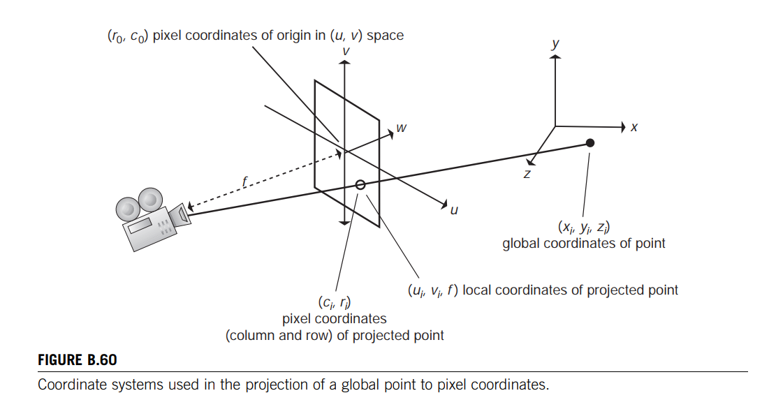
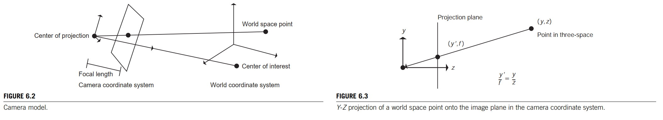
The two-dimensional image coordinates are a mapping of the local two-dimensional image plane of the camera located a distance $f$ in front of the camera (Eq. B.171). 从摄像机空间下的坐标到屏幕坐标
$$
\begin{cases}
c_i - c_0 = s_uu_i\\
r_i - r_0 = s_vv_i
\end{cases}
\tag{B.171}
$$
The image plane is located relative to the three-dimensional local coordinate system $(u, v, w)$ of the camera (Figure B.60).
The imaging of a three-dimensional point is approximated using a pinhole camera model. The three-dimensional local coordinate system of the camera is related to the three dimensional global coordinate system by a rotation and translation (Eq. B.172); 摄像机坐标系通过旋转R和平移T变成世界坐标系,也就是说世界坐标系下的点坐标经过R和T可以变成摄像机坐标系的点坐标
$$
\begin{bmatrix}
u_i \\ v_i \\ f
\end{bmatrix}
=
R\begin{bmatrix}
x_i \\ y_i \\ z_i
\end{bmatrix} + T
\tag{B.172}
$$
$$
R = \begin{bmatrix}
R_0 \\ R_1 \\ R_2
\end{bmatrix}
=
\begin{bmatrix}
r_{0,0} & r_{0,1} & r_{0,2}\\
r_{1,0} & r_{1,1} & r_{1,2}\\
r_{2,0} & r_{2,1} & r_{2,2}
\end{bmatrix}
$$
$$
T = \begin{bmatrix}
t_0 \\ t_1 \\ t_2
\end{bmatrix}
$$
the origin of the camera’s local coordinate system is assumed to be at the focal point of the camera. The three-dimensional coordinates are related to the two-dimensional coordinates by the transformation to be determined.
Equation B.173 expresses the relationship between a pixel’s column and row number and the global coordinates of the point. 点在屏幕空间下的坐标和世界空间下的坐标关系
$$
\frac{u_i}{f} = \frac{c_i - c_0}{s_uf} = \frac{c_i - c_0}{f_u} = \frac{R_0 \cdot [x_iy_iz_i] + t_0}{R_2 \cdot [x_iy_iz_i] + t_2}
$$
$$
\frac{v_i}{f} = \frac{r_i - r_0}{s_vf} = \frac{r_i - r_0}{f_v} = \frac{R_1 \cdot [x_iy_iz_i] + t_1}{R_2 \cdot [x_iy_iz_i] + t_2}
\tag{B.173}
$$
These equations are rearranged and set equal to zero in Equation B.174. They can be put in the form of a system of linear equations (Eq. B.175) so that the unknowns are isolated (Eq. B.176) by using substitutions common in camera calibration (Eqs. B.176 and B.177). 现在未知数全跑$W$上了
$$
(c_i-c_0)(R_2 \cdot [x_iy_iz_i] + t_2) - f_u(R_0 \cdot [x_iy_iz_i] + t_0) = 0\\
(r_i-r_0)(R_2 \cdot [x_iy_iz_i] + t_2) - f_v(R_1 \cdot [x_iy_iz_i] + t_1) = 0
\tag{B.174}
$$
$$
AW = 0 \Longleftrightarrow
\begin{bmatrix}
-x_1 & -y_1 & -z_1 & 0 & 0 & 0 & r_1x_1 & r_1y_1 & r_1z_1 & -1 & 0 & r_1 \\
0 & 0 & 0 & -x_1 & -y_1 & -z_1 & c_1x_1 & c_1y_1 & c_1z_1 & 0 & -1 & c_1
\end{bmatrix}
\begin{bmatrix}
w_0\\w_1\\w_2\\w_3\\ \cdots \\w_{11}
\end{bmatrix}
=0
\tag{B.175}
$$
$$
\begin{aligned}
&W_0 = f_uR_0 + c_0R_2 = [w_0 w_1 w_2]^T\\
&W_3 = f_vR_1 + r_0R_2 = [w_3 w_4 w_5]^T\\
&W_6 = R_2 = [w_6 w_7 w_8]^T\\
&w_9 = f_ut_0 + c_0t_2\\
&w_{10} = f_vf_1 + r_0t_2\\
&w_{11} = t_2
\end{aligned}
\tag{B.176}
$$
$$
W = \begin{bmatrix}
w_0 & w_1 & w_2 & w_3 & w_4 & w_5 & \cdots & w_{11}
\end{bmatrix}^T
\tag{B.177}
$$
Temporarily dividing through by $t_2$ ensures that $t_2 \neq 0.0$ and therefore that the global origin is in front of the camera. This step results in Equation B.178, where $A’$ is the first $11$ columns of $A$; $B’$ is the last columnof $A$; and $W’$ is the first $11$ rows of $W$. 不是很懂,但感觉是为了方便最小二乘计算
Typically, enough points are captured to ensure an overdetermined system. Then a least squares method, such as singular value decomposition, can be used to find the $W’$ that satisfies Equation B.179. 找到最优的 $W’$,使得 $A’W’$ 与 $-B’$ 距离最近
$$
A’W’ + B’ = 0
\tag{B.178}
$$
$$
\underset{w}{min} ||A’W’ + B’||
\tag{B.179}
$$
$W’$ is related to $W$ by Equation B.180, and the camera parameters can be recovered by undoing the substitutions made in Equation B.176 by Equation B.181.
$$
W = \begin{bmatrix}
W_0 \\ W_3 \\ W_6 \\ W_9 \\ W_{10} \\ W_{11}
\end{bmatrix}
=
\frac{1}{||W_6’||} \times
\begin{bmatrix}
W_0’ \\ W_3’ \\ W_6’ \\ W_9’ \\ W_{10}’ \\ W_{11}’
\end{bmatrix}
\tag{B.180}
$$
$$
\begin{aligned}
&c_0 = W_0^TW_6\\
&r_0 = W_1^TW_6\\
&f_u = - ||W_0 - c_0W_6||\\
&t_0 = (w_9 - c_0) / f_u\\
&t_1 = (w_{10} - r_0) / f_v\\
&t_2 = w_{11}\\
&R_0 = (W_0 - c_0W_6) / f_u\\
&R_1 = (W_3 - r_0W_6) / f_v\\
&R_2 = W_6
\end{aligned}
\tag{B.181}
$$
Because of numerical imprecision, the rotation matrix recovered may not be orthonormal正交矩阵, so it is best to reconstruct the rotation matrix first (Eq. B.182),
$$
\begin{aligned}
&R_0 = (W_0’ - c_0W_6’) / f_u\\
&R_1 = (W_3’ - r_0W_6’) / f_v\\
&R_2 = W_6’
\end{aligned}
\tag{B.182}
$$
massage it into orthonormality, and then use the new rotation matrix to generate the rest of the parameters (Eq. B.183).
$$
\begin{aligned}
&c_0 = W_0^TR_2\\
&r_0 = W_1^TR_2\\
&f_u = - ||W_0 - c_0R_2||\\
&f_v = ||W_3 - r_0R_2||\\
&t_0 = (w_9 - c_0) / f_u\\
&t_1 = (w_{10} - r_0) / f_v\\
&t_2 = w_{11}\\
\end{aligned}
\tag{B.183}
$$
…
感觉讲的不是很懂
Three-dimensional position reconstruction
The greater the orthogonality of the two views, the better the chance for an accurate reconstruction.
If the position and orientation of each camera are known with respect to the global coordinate system, along with the position of the image plane relative to the camera, then the images of the point to be reconstructed $(I_1, I_2)$ can be used to locate the point, $P$, in three-space (Figure 6.4).
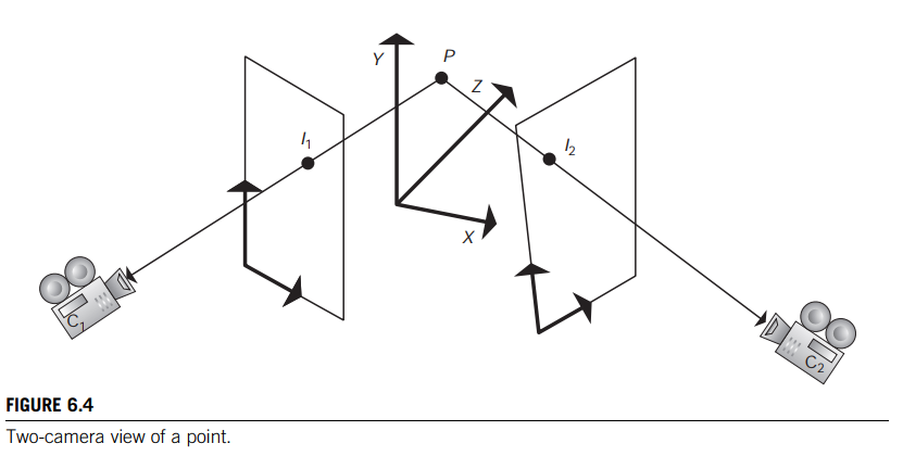
Using the location of a camera, the relative location of the image plane, and a given pixel location on the image plane, the user can compute the position of that pixel in world coordinates. Once that is known, a vector from the camera through the pixel can be constructed in world space for each camera (Eqs. 6.1 and 6.2).
$$
\begin{aligned}
&C_1 + k_1(I_1 - C_1) = P\\
&C_2 + k_2(I_2 - C_2) = P\\
&C_1 + k_1(I_1 - C_1) = C_2 + k_2(I_2 - C_2)
\end{aligned}
$$
Three equations and two unknows, so we can get $k_1, k_2$ easily. However, In practice, these two equations will not exactly intersect, although if the noise in the system is not excessive, they will come close.
So, in practice, the points of closest encounter must be found on each line. This requires that a $P_1$ and a $P_2$ be found such that $P_1$ is on the line from Camera 1, $P_2$ is on the line from Camera 2, and $P_2P_1$ is perpendicular to each of the two lines (Eqs. 6.3 and 6.4).
$$
\begin{aligned}
&(P_2 - P_1) \cdot (I_1 - C_1) = 0\\
&(P_2 - P_1) \cdot (I_2 - C_2) = 0
\end{aligned}
\tag{6.3}
$$
Once the points $P_1$ and $P_2$ have been calculated, the midpoint of the chord between the two points can be used as the location of the reconstructed point.
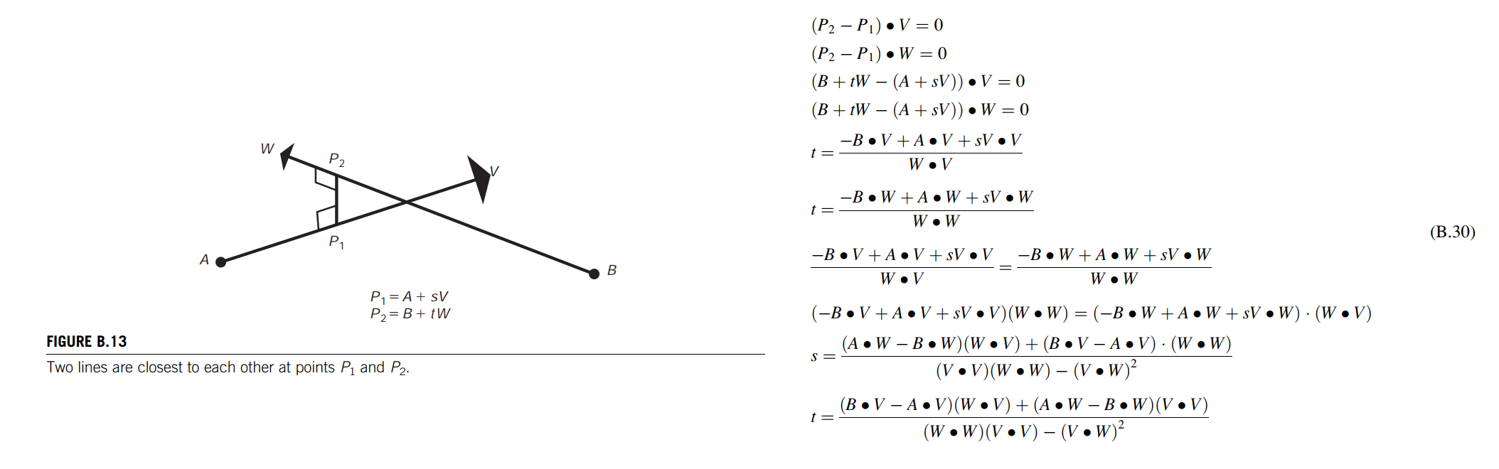
B.2.6 Closest point between two lines in three-space
The intersection of two lines in three-space often needs to be calculated. Because of numerical imprecision, the lines rarely, if ever, actually intersect in three-space. As a result, the computation that needs to be performed is to find the two points, one from each line, at which the lines are closest to each other.
The points $P_1$ and $P_2$ at which the lines are closest form a line segment perpendicular to both lines (Figure B.13).
They can be represented parametrically as points along the lines, and then the parametric interpolants can be solved for by satisfying the equations that state the requirement for perpendicularity (Eq. B.30)
Multiple markers
Multiple cameras
To reconstruct the three-dimensional position of a marker, the system must detect and identify the marker in at least two images.
Fitting to the skeleton
Once the motion of the individual markers looks smooth and reasonable, the next step is to attach them to the underlying skeletal structure that is to be controlled by the digitized motion.
One source of the problem is that the markers are located not at the joints of the performers, but outside the joints at the surface. This means that the point being digitized is displaced from the joint itself.
One solution is to put markers on both sides of the joint. With two marker locations, the joint can be interpolated as the midpoint of the chord between the two markers. While effective for joints that lend themselves to this approach, the approach does not work for joints that are complex or more inaccessible (such as the hip, shoulder, and spine), and it doubles the number of markers that must be processed.
A little geometry can be used to calculate the displacement of the joint from the marker. A plane formed by three markers can be used to calculate a normal to a plane of three consecutive joints, and this normal can be used to displace the joint location.
Output from motion capture systems
.bvh/.asf/.asm
Manipulating motion capture data
There are various ways to manipulate mocap data. Some are straightforward applications of standard signal processing techniques while others are active areas of research. These techniques hold the promise of enabling motion libraries to be constructed along with algorithms for editing the motions, mapping the motions to new characters, and combining the motions into novel motions and or longer motion sequences.
Processing the signals
The values of an individual parameter of the captured motion (e.g., a joint angle) can be thought of, and dealt with, as a time-varying signal.
Motion signal processing considers how frequency components capture various qualities of the motion [1]. The lower frequencies of the signal are considered to represent the base activity (e.g., walking) while the higher frequencies are the idiosyncratic movements of the specific individual (e.g., walking with a limp). the signal is successively convolved with expanded versions of a filter kernel (e.g., 1/16, 1/4, 3/8, 1/4, 1/16). The frequency bands are generated by differencing the convolutions. Gains of each band are adjusted by the user and can be summed to reconstruct a motion signal.滤波器得到不同频率的信号
Motion wraping warps the signal in order to satisfy user-supplied key-frame-like constraints[9]. For example, The original signal is $y(t)$ and the key frames are given as a set of $(y_i, t_i)$ pairs. In addition, there is a set of time warp constraints $(t_j, t_j’)$.
warping procedure:
- creates a time warp mapping $t = g(t’)$ by interpolating through the time warp constraints.
- creates a motion curve warping, $\theta(t) = f(\theta, t)$.
- the function is created by scaling and/or translating the original curve to satisfy the key-frame constraints $\theta’(t) = a(t)\theta(t) + b(t)$ whether to scale or translate can be user-specified.
- Once the functions $a(t)$ and $b(t)$ for the key frames are set, the functions $a(t)$ and $b(t)$ can be interpolated throughout the time span of interest.
- Combined, these functions establish a function $\theta(t’)$ that satisfies the key-frame and time warp constraints by warping the original function.
其实就像一个$\sin t$ 函数,被用户指定更改了频率,振幅,相位等一系列参数一样, like $3\sin (2t + \frac{\pi}{4})$
Retargeting the motion
What happens if the synthetic character doesn’t match the dimensions (e.g., limb length) of the captured subject?
One solution is to map the motion onto the mismatched synthetic character and then modify it to satisfy important constraints.
Important constraints include such things as avoiding foot penetration of the floor, avoiding self-penetration, not letting feet slide on the floor when walking, and so forth.
A new motion is constructed, as close to the original motion as possible, while enforcing the constraints.
Finding the new motion is formulated as a space–time, nonlinear constrained optimization problem.
[2] Gleicher M. Retargeting Motion to New Characters. In: Cohen M, editor. Proceedings of SIGGRAPH 98,Computer Graphics, Annual Conference Series. Orlando, Fla.: Addison-Wesley; July 1998. p. 33–42. ISBN 0-89791-999-8.
Combining motions
The ability to assemble motion segments into longer actions makes motion capture a much more useful tool for the animator.
More natural transitions between segments are possible by blending the end of one segment into the beginning of the next one. Such transitions may look awkward unless the portions to be blended are similar. Similarity can be defined as the sum of the differences over all DOFs over the time interval of the blend.
Automatic techniques to identify the best subsegments for transitions is the subject of current research [4].
有时候融合两个motion clip的时候,比如walk和run,会发现walk是从左到右,run从右到左,如果直接blend会滑步,这是因为没有运动对齐,此时需要facing frame坐标系来解决这个问题—A special coordinate system that moves horizontally with the character with one axis pointing to the “facing direction” of the character,一般情况下这个坐标系是根关节RootJoint在地上的投影,这个坐标系的z轴指向的是Character速度的方向或者朝向(默认绝对坐标系是y-up)
[4] Kovar L, Gleicher M. Flexible Automatic Motion Blending with Registration Curves. In: Breen D, Lin M, editors. Symposium on Computer Animation. San Diego, Ca.: Eurographics Association; 2002. p. 214–24.
Recent research has produced techniques such as motion graphs that identify good transitions between segments in a motion database [3] [5] [7]. When the system is confronted with a request for a motion task, the sequence of motions that satisfies the task is constructed from the segments in the motion capture database.
motion graph 就是现在游戏开发中常说的状态机_2002,可以实现用户可交互的动画,但这种方法有个缺点,就是对用户的响应比较慢,需要播放完当前的motion clip后才进行下一个节点的运动。
对这种方法的改进就是motion matching_2016,启发自motion fields_2010方法,此方法不是按照motion clip的切换这种视角来进行交互动画,而是每一帧的姿态都是独立的,根据用户输入,环境信息,从motion database中找到下一帧最适合的pose,然后进行平滑的transition。很明显motion matching的方法对用户输入响应及时,但是对内存和计算的需求很大,且在此方法中,两个pose之间的距离函数一定要设计好,或者feature要extract的不错,才能找到比较不错的nearest neighbor。
[3] Kovar L, Gleicher M, Pighin F. Motion Graphs, In: Proceedings of SIGGRAPH 2002, Computer Graphics, Annual Conference Series. San Antonio, Tex.; July 23–26,; 2002. p. 473–82.
[5] Lee J, Chai J, Reitsma P, Hodgins J, Pollard N. Interactive Control of Avatars Animated with Human Motion Data, In: Computer Graphics, Proceedings of SIGGRAPH 2002, Annual Conference Series. San Antonio, Tex.; July 23–26, 2002. p. 491–500.
[7] Reitsma P, Pollard N. Evaluating Motion Graphs for Character Navigation. In: Symposium on Computer Animation. Grenoble, France. p. 89–98.
Chapter summary
Current research involves extracting motion capture data from markerless video. This has the potential to free the subject from instrumentation constraints and make motion capture even more useful.
深度学习—单目视频三维角色重建..

